####################################
###### Assignment to Genes ##########
####################################
# find "outlier genes" by comparing genomic regions identified as outliers with the locations of
# genes annotated in a GFF (General Feature Format) file.
# Reference genome file
gff <- read.delim("/home/tahirali/RAMSES_mount/tali/qbio/Practical_Day_3/At_gff/GFF_final_with_annotation_2_gff", header = FALSE)
# Read the GFF file, which contains genomic annotations (genes, exons, etc.). The file does not have column headers initially.
# Add column names to the data frame for easier access
colnames(gff) <- c("model_name", "chromosome", "source", "type", "start", "end", "score", "strand", "phase", "attributes")
# Assign meaningful column names to the data (e.g., model name, chromosome, feature type, start/end positions)
# Remove the first row that is without any data (probably an empty row)
gff <- gff[-1,]
# Convert the 'start' and 'end' columns to numeric data types (they might be read as factors or characters initially)
gff$start <- as.numeric(as.character(gff$start))
gff$end <- as.numeric(as.character(gff$end))
# Filter the data to exclude non-gene types (e.g., UTRs, introns, exons, etc.)
# We focus only on the main gene annotations.
filtered_annotation <- subset(gff, !(type %in% c("UTR", "intron", "exon", "five_prime_UTR", "three_prime_UTR", "chromosome")))
# The 'type' column in the GFF file contains different feature types like UTR, exon, intron, etc. We filter out those we're not interested in.
# Preparation of outlier data
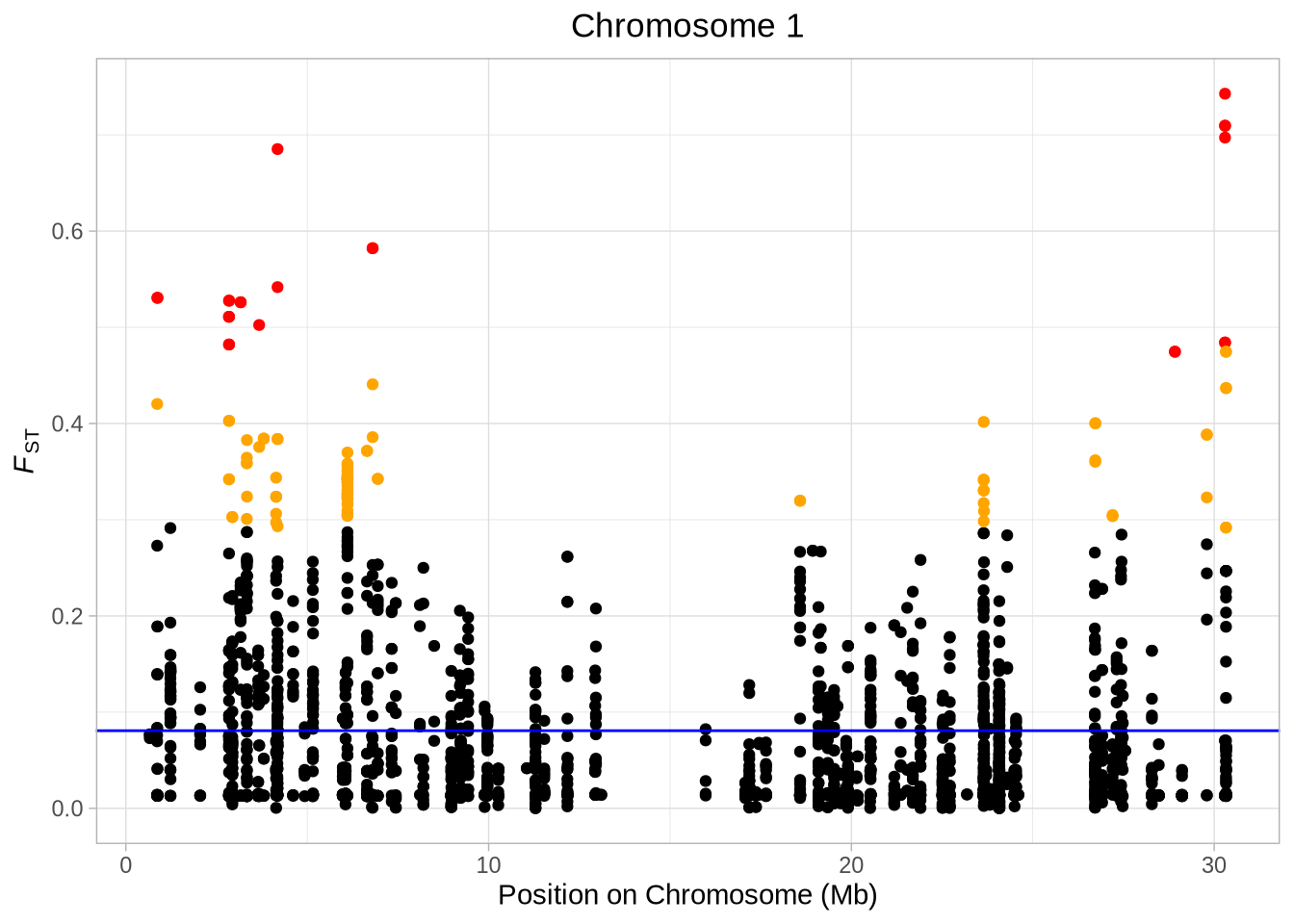
# 95% outlier
# Rename the 6th column to match the naming convention (standardizing column names)
colnames(out_95)[6] <- "ESP_SWE_fst"
# Remove rows with 99% outliers, as we're focusing on the 95% outliers here.
outs_95 <- out_95[out_95$outlier_99 != "Outlier", ]
# The "outlier_99" column in the 'out_95' dataset indicates whether a row is an outlier. We filter out rows marked as "Outlier" in that column.
# 99% outlier
# Rename the 6th column to match the naming convention for consistency
colnames(out_99)[6] <- "ESP_SWE_fst"
out_99 # View the data for 99% outliers
# Manually assign chromosome information to 'out_99' since it might be missing or inconsistent.
out_99$chromosome <- c("Chr1")
# In this example, we are assuming the outliers in 'out_99' are located on "Chr1". In real data, this would be dynamically assigned based on actual information.
# Search for overlaps between outlier regions and gene regions
# Create a GRanges object for the gene annotations from the filtered GFF file.
# GRanges is a specialized object from the GenomicRanges package for storing genomic ranges efficiently.
gene_ranges <- GRanges(
seqnames = filtered_annotation$chromosome, # Chromosome information
ranges = IRanges(start = filtered_annotation$start, end = filtered_annotation$end) # Genomic range (start and end positions)
)
# Create a GRanges object for the outlier regions (95% outliers)
outlier_ranges_95 <- GRanges(
seqnames = outs_95$chromosome, # Chromosome information for the 95% outliers
ranges = IRanges(start = outs_95$start, end = outs_95$stop) # Outlier start and end positions
)
# Create a GRanges object for the outlier regions (99% outliers)
outlier_ranges <- GRanges(
seqnames = out_99$chromosome, # Chromosome information for the 99% outliers
ranges = IRanges(start = out_99$start, end = out_99$stop) # Outlier start and end positions
)
# Find overlaps between the outlier regions and gene regions
# 'findOverlaps' function identifies overlapping ranges between two GRanges objects
overlaps_95 <- findOverlaps(outlier_ranges_95, gene_ranges, type = "any", select = "all", ignore.strand = TRUE)
overlaps <- findOverlaps(outlier_ranges, gene_ranges, type = "any", select = "all", ignore.strand = TRUE)
# These lines find the overlaps between the 95% and 99% outlier regions and the gene regions. It returns the indices of overlapping genes.
# Extract the indices of overlapping genes for the 95% and 99% outlier regions
overlapping_genes_indices_95 <- subjectHits(overlaps_95)
overlapping_genes_indices <- subjectHits(overlaps)
# 'subjectHits' extracts the indices of genes from the filtered annotation that overlap with the outlier regions.
# Retrieve the actual gene information for the overlapping genes based on the indices.
overlapping_genes_95 <- filtered_annotation[overlapping_genes_indices_95, ]
overlapping_genes <- filtered_annotation[overlapping_genes_indices, ]
# These lines fetch the actual gene annotations (rows of the filtered GFF file) that correspond to the overlapping regions.
##############################################################################################################
### Compare diversity statistics for each population within defense-related genes versus the whole genome ###
##############################################################################################################
vcf_full <- readVcf("1001genomes_snp-short-indel_only_ACGTN_Dp10GQ20Q30_NoIndel_Bialleleic_80PcMissing_80SwEs.vcf.recode.vcf.gz")
chromosomes <- seqlevels(vcf) # Get chromosome names
# Calculate start and end positions for each chromosome
chromosome_ranges <- data.frame(CHROM = character(), Start = numeric(), End = numeric(), stringsAsFactors = FALSE)
for (chrom in chromosomes) {
positions <- start(vcf[seqnames(vcf) == chrom])
chromosome_ranges <- rbind(chromosome_ranges, data.frame(CHROM = chrom, Start = min(positions), End = max(positions)))
}
print(chromosome_ranges)
#CHROM Start End
#1 1 2784 30422721
#2 2 24180 19697399
#3 3 1705 23459492
#4 4 1552 18584482
#5 5 115 26974567
# Define genomic ranges for chromosomes to be analyzed
# These ranges correspond to the positions on the chromosomes of interest
chr1start <- 2784; chr1end <- 30422721
chr2start <- 24180; chr2end <- 19697399
chr3start <- 1705; chr3end <- 23459492
chr4start <- 1552; chr4end <- 18584482
chr5start <- 115; chr5end <- 26974567
# Example: chromosome 1 (use all the variants across the whole genome)
At_full_Chr <- suppressMessages(
readVCF("1001genomes_snp-short-indel_only_ACGTN_Dp10GQ20Q30_NoIndel_Bialleleic_80PcMissing_80SwEs.vcf.recode.vcf.gz", numcols=189, tid="1", frompos = chr1start, topos = chr1end, include.unknown = TRUE)
)
# Define populations using metadata (Ensure you have the "pop1.txt" file with the correct format)
population_info <- read_delim("pop1.txt", delim = "\t") # Two columns: sample ID and population
populations <- split(population_info$sample, population_info$pop) # Create list of populations
At_full_Chr <- set.populations(At_full_Chr, populations, diploid = TRUE) # Assign populations to PopGenome object
# Define sliding windows for analysis
window_size <- 100; window_jump <- 50
strt <- chr1start; end <- chr1end # Set start and end for chromosome 1 (update for others)
window_start <- seq(from = strt, to = end, by = window_jump) # Generate start positions for sliding windows
window_stop <- window_start + window_size # Calculate stop positions
window_start <- window_start[window_stop < end] # Remove windows exceeding chromosome length
window_stop <- window_stop[window_stop < end]
windows <- data.frame(start = window_start, stop = window_stop, mid = window_start + (window_stop - window_start) / 2)
# Transform data into sliding windows and calculate statistics
At_full_sw <- suppressMessages(
sliding.window.transform(At_full_Chr, width = 100, jump = 50, type = 2)
)
####### Calculating sliding window estimates of nucleotide diversity and differentiation #####
# Step 1: Calculating nucleotide diversity (pi), FST, and d_XY_ (absolute nucleotide divergence between populations).
# The diversity.stats function calculates various diversity statistics including pi and sets up for d_XY_ calculation.
At_full_sw <- suppressMessages(
diversity.stats(At_full_sw, pi = TRUE)
) # Calculates nucleotide diversity (pi) and sets up d_XY_
At_full_sw <- suppressMessages(
neutrality.stats(At_full_sw)
) # Calculates neutrality statistics
# Checking neutrality for populations (1 and 2), # Uncomment if you want to print header
# head(get.neutrality(At_full_sw)[[1]]) # Population 1
# head(get.neutrality(At_full_sw)[[2]]) # Population 2
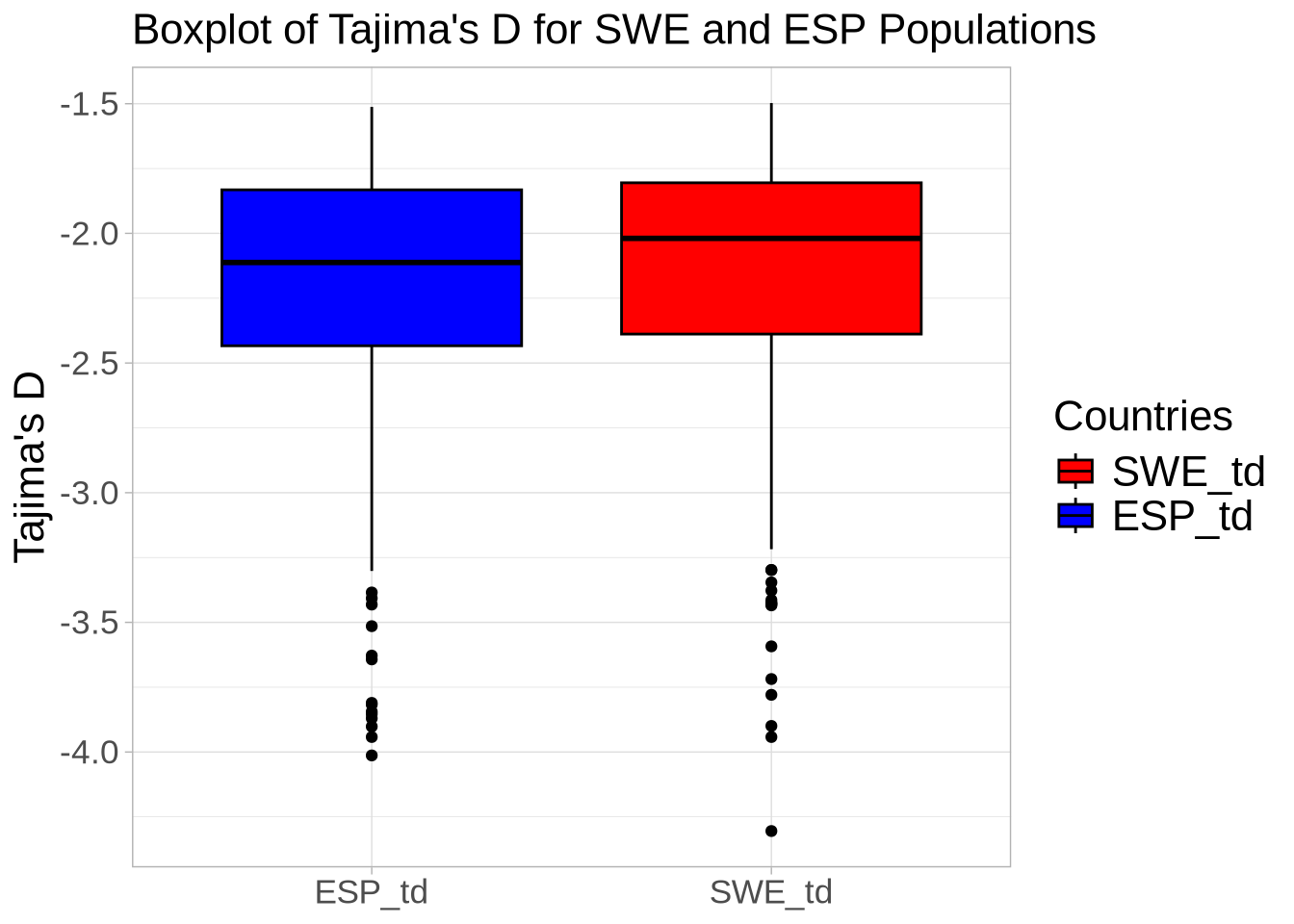
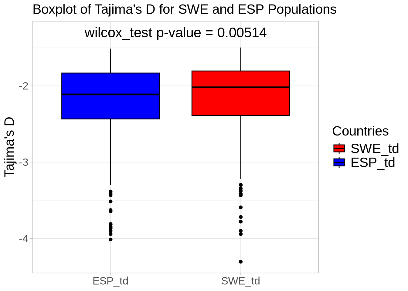
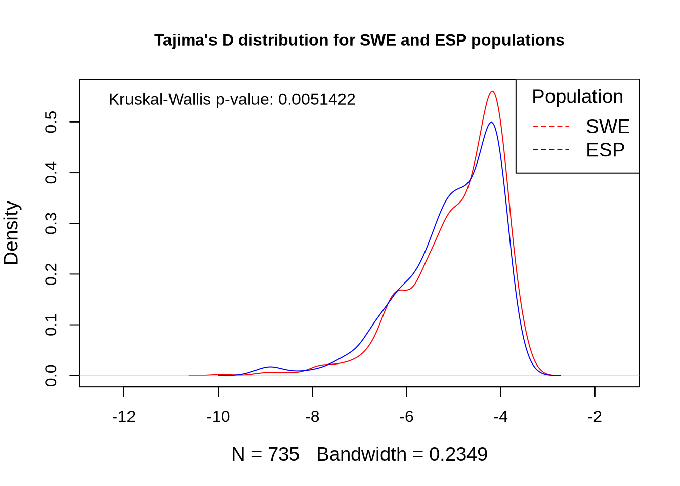
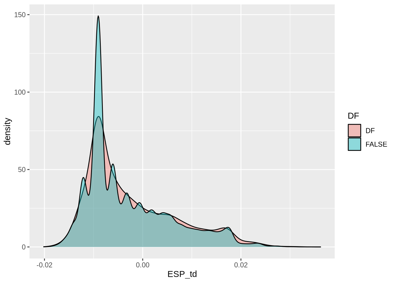
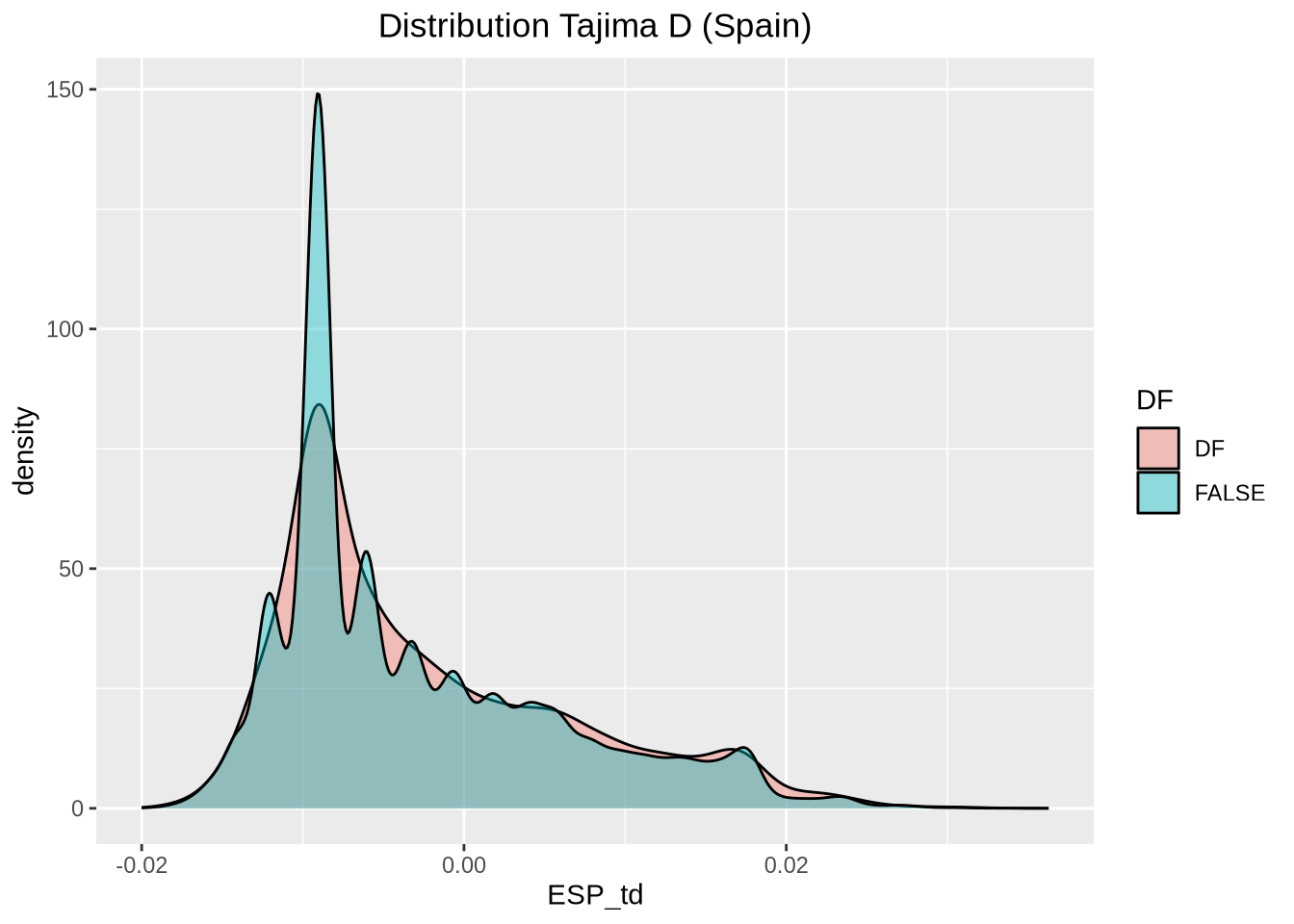
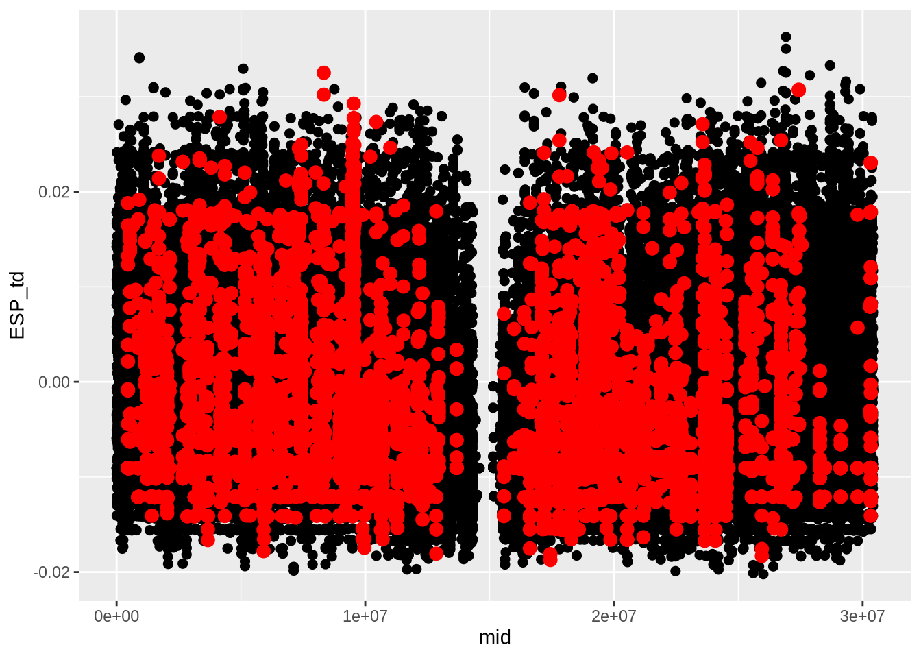
# Extract Tajima's D and adjust for scale
td_full <- At_full_sw@Tajima.D / 100 # Divide by 100 to scale it
# Assign population names to the Tajima's D data
colnames(td_full) <- paste0(names(populations), "_td")
# Wrap functions in `suppressMessages()` and/or `suppressWarnings()
# For functions that print messages explicitly:
# Step 2: Calculate FST using nucleotide data (mode = "nucleotide" for sliding window averages)
At_full_sw <- suppressMessages(
F_ST.stats(At_full_sw, mode = "nucleotide")
) # Calculate FST for nucleotide data
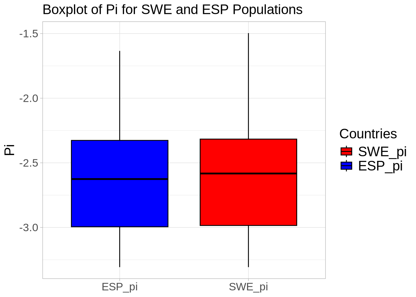
# Step 3: Extract statistics for visualization
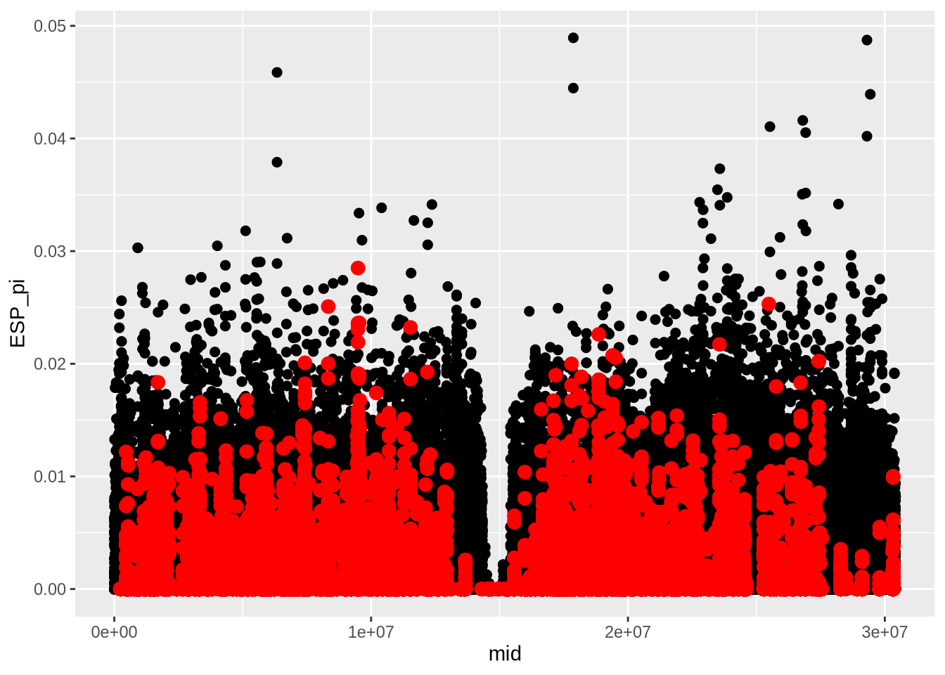
# Extract nucleotide diversity and correct for window size (100 bp)
nd_full <- At_full_sw@nuc.diversity.within / 100 # Nucleotide diversity (pi)
colnames(nd_full) <- paste0(names(populations), "_pi") # Set population names for diversity data
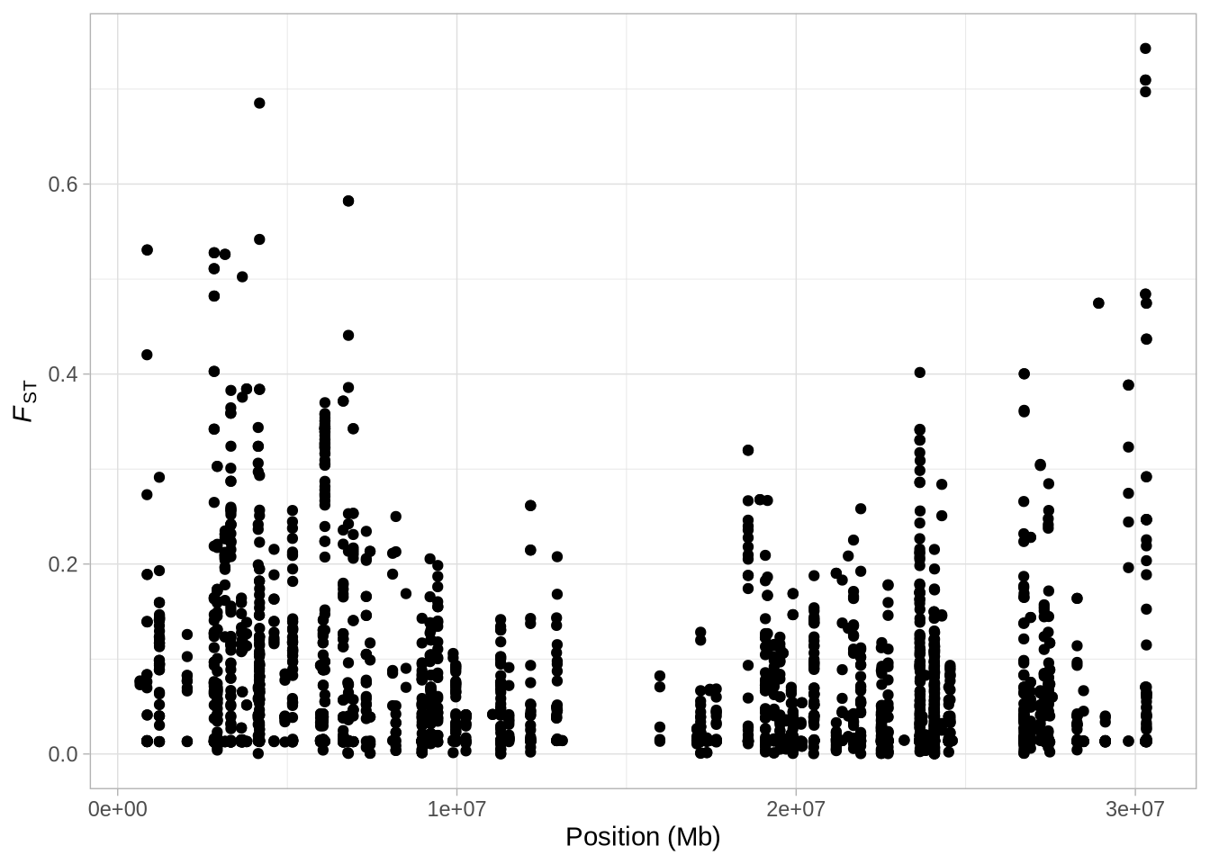
# Extract FST values and transpose the matrix for easier comparison
fst_full <- t(At_full_sw@nuc.F_ST.pairwise) # Pairwise FST, transposed to have windows in rows
# Correct column names for FST (pairwise comparison names)
# Modify Fst column names
x <- colnames(fst_full)
for (i in seq_along(populations)) {
x <- sub(paste0("pop", i), names(populations)[i], x)
}
colnames(fst_full) <- paste0(sub("/", "_", x), "_fst")
# head(fst_full) # Uncomment if you want to print header
# Step 4: Combine all statistics into a single data frame for visualization
library(tibble)
At_data_full <- as.tibble(data.frame(windows, nd_full, fst_full, td_full)) # Add Tajima's D (td) to the final dataset
# head(At_data_full) # Uncomment if you want to print header
# Filter out rows where any column has zero or NA values
filtered_stats_full <- At_data_full %>%
filter(
!if_any(everything(), ~ . == 0 | is.na(.))
)
# Print the filtered tibble
head(filtered_stats_full, n = 5)
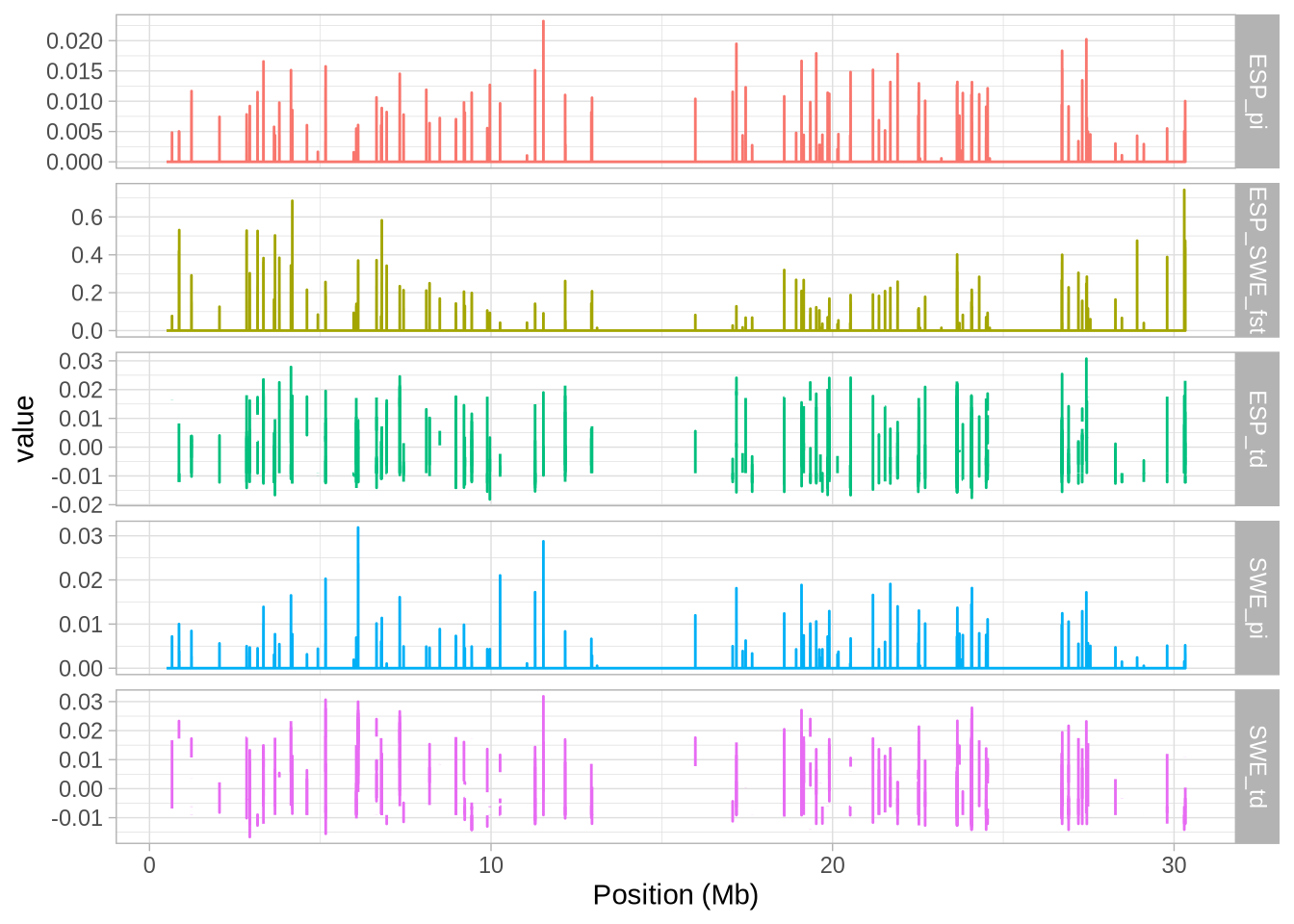
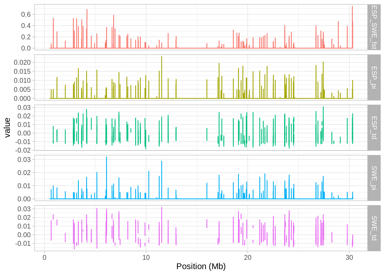
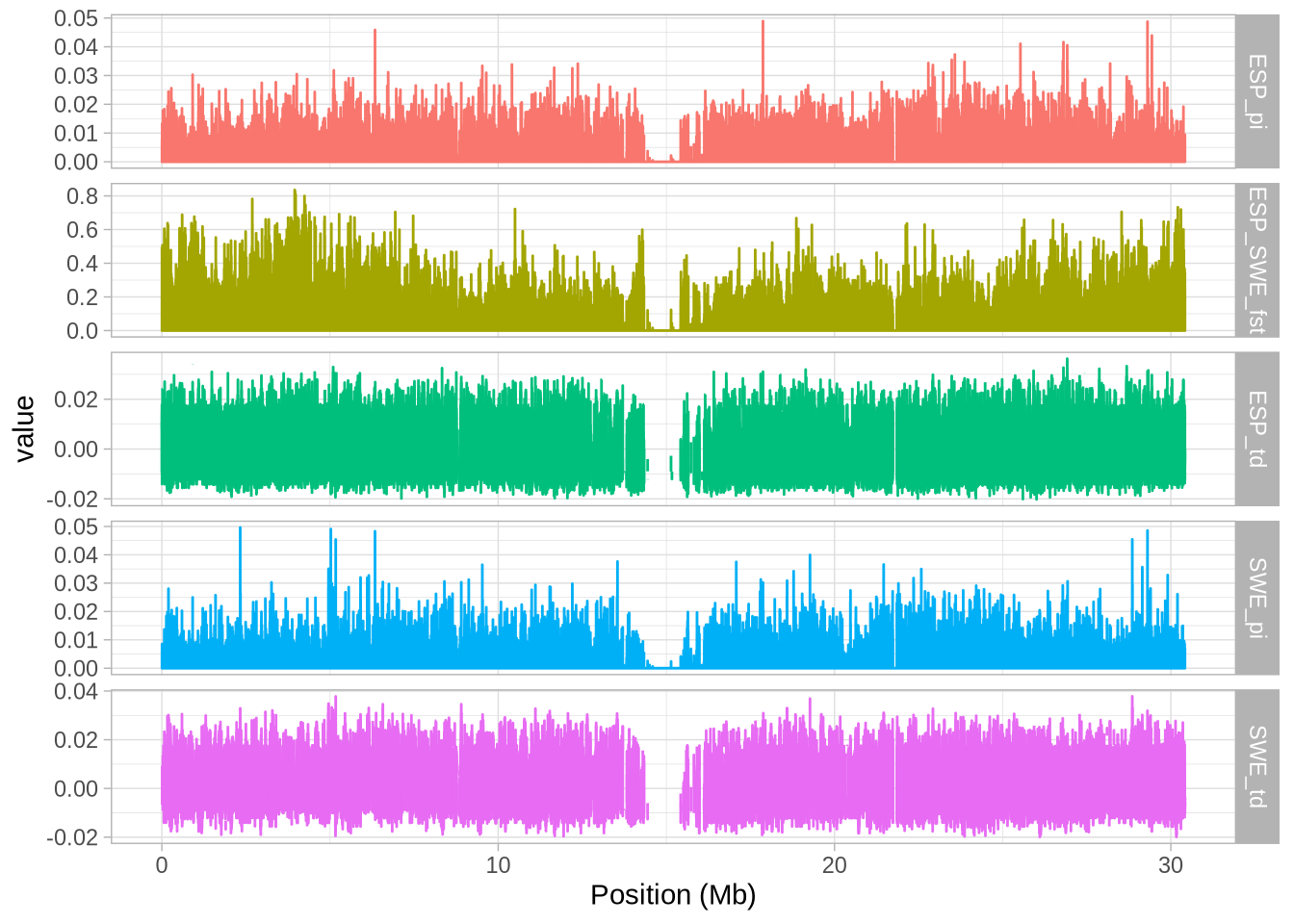
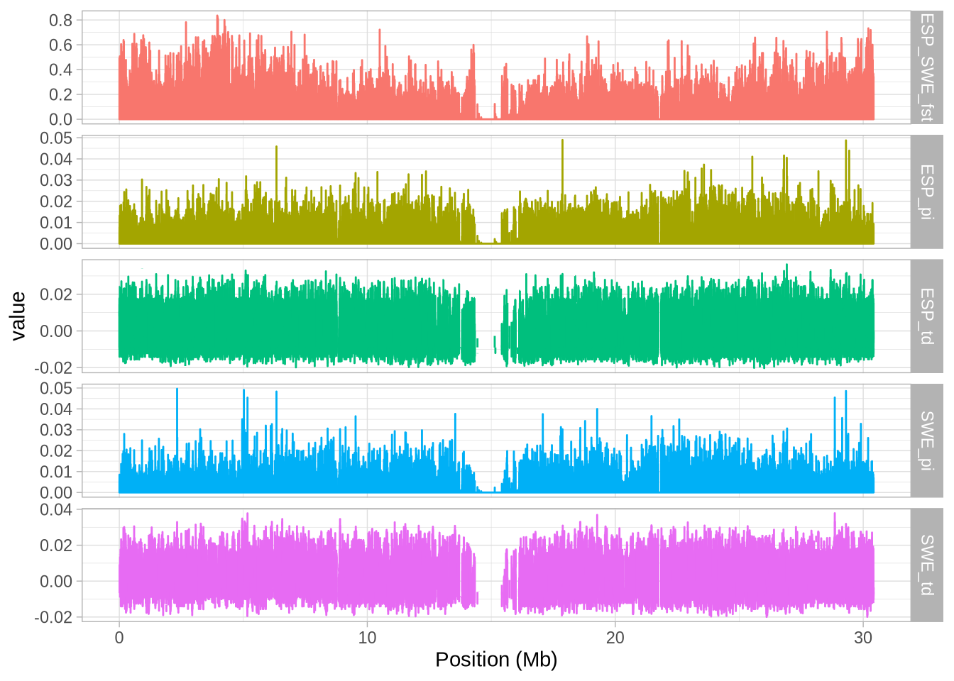
###########################
## Create a Facet plot ----
###########################
# To set Fst values smaller than zero to zero using dplyr and %>%, we use mutate and across
hs_full <- At_data_full %>%
select(mid, ESP_pi, SWE_pi, ESP_td, SWE_td, ESP_SWE_fst) %>% # Select relevant columns
mutate(across(c(ESP_SWE_fst), ~ ifelse(. < 0, 0, .))) # Set negative Fst values to 0
# Use gather to reshape the data for easier plotting
hs_g_full <- gather(hs_full, -mid, key = "stat", value = "value")
# 'gather' collapses data by statistics ('stat'), keeping 'mid' as a fixed column
# Create a plot with facets to visualize the data
a_full <- ggplot(hs_g_full, aes(mid/10^6, value, colour = stat)) + geom_line()
a_full <- a_full + facet_grid(stat~., scales = "free_y") # Split data by 'stat' into separate panels
a_full <- a_full + xlab("Position (Mb)") # Label the x-axis
a_full + theme_light() + theme(legend.position = "none") # Use a light theme and remove legend