Spatial Sampling and Ecological Inference: A Hands-On Spatial Point Pattern Analysis

Case Study of Pakistan: Spider Web dataset

Author

Dr Tahir Ali | AG de Meaux | TRR341 Ecological Genomics | University of Cologne

Introduction

This session introduces the fundamentals of spatial sampling and ecological inference using a case study of spider web observations from Pakistan. Participants learn how to load, clean, and project spatial datasets (species occurrences, boundaries, roads, and waterways), and create maps to visualize sampling patterns at national and regional scales.

Using kernel density estimation and spatial point-pattern analysis, the tutorial explores whether spider observations are randomly distributed or clustered. Statistical methods—including the Clark–Evans test, Ripley’s K function, pair correlation function, and Moran’s I—are applied to detect clustering, identify its spatial scale, and quantify spatial autocorrelation.

The exercise also demonstrates how sampling bias related to accessibility (e.g., proximity to roads or rivers) can influence ecological data and how such biases can be diagnosed and considered in ecological interpretation. 🌍🕷️📊

1. Load data

Data used in this workshop can be downloaded from: https://github.com/tahirali-biomics/spatial-ecology-workshop/

Load necessary libraries for spatial analysis (sf, ggplot2, spatstat, etc.)
Read spider presence data from CSV with comma decimals (European format)
Convert coordinates to numeric and remove duplicate records
Load Pakistan boundary, roads, and waterways shapefiles
Transform all data to UTM zone 43N (meters) for accurate distance calculations

Code

cat("\n=== LOADING SPIDER DATA ===\n")


=== LOADING SPIDER DATA ===

Code

library(sf)
library(terra)
library(ggplot2)
library(dplyr)
library(viridis)
library(MASS)

# Load spider presences
spiders <- read.csv2("/run/media/tahirali/Expansion/github/spatial-ecology-workshop/data/presence/spider_coords.csv",
                     header = TRUE)

# Convert comma decimals to numeric
spiders$X <- as.numeric(gsub(",", ".", spiders$X))
spiders$Y <- as.numeric(gsub(",", ".", spiders$Y))

# Remove duplicates
spiders <- distinct(spiders)
cat("Loaded", nrow(spiders), "unique spider records\n")

Loaded 93 unique spider records

Code

# Convert to sf object
sp_points <- st_as_sf(spiders, coords = c("X", "Y"), crs = 4326)

# Transform to UTM (meters) for distance calculations
sp_utm <- st_transform(sp_points, 32643) # UTM zone 43N for Pakistan

# Extract coordinates
coords <- st_coordinates(sp_utm)
spiders$x <- coords[,1]
spiders$y <- coords[,2]

# ==============================================================================
# LOAD PAKISTAN ADMIN BOUNDARY
# Source:https://data.humdata.org/dataset/cod-ab-pak
# ==============================================================================
cat("\n=== LOADING PAKISTAN BOUNDARY ===\n")


=== LOADING PAKISTAN BOUNDARY ===

Code

pakistan_boundary <- st_read("/run/media/tahirali/Expansion/github/spatial-ecology-workshop/data/boundaries/pakistan_admin.shp")

Reading layer `pakistan_admin' from data source 
  `/run/media/tahirali/Expansion/github/spatial-ecology-workshop/data/boundaries/pakistan_admin.shp' 
  using driver `ESRI Shapefile'
Simple feature collection with 8 features and 11 fields
Geometry type: MULTIPOLYGON
Dimension:     XY
Bounding box:  xmin: 60.89944 ymin: 23.70292 xmax: 77.84308 ymax: 37.09701
Geodetic CRS:  WGS 84

Code

pakistan_boundary <- st_transform(pakistan_boundary, 32643)
cat("✓ Pakistan boundary loaded\n")

✓ Pakistan boundary loaded

Code

# ==============================================================================
# LOAD FULL ROADS NETWORK - CORRECTED PATH
# Source: HDX Pakistan Roads: https://data.humdata.org/dataset/hotosm_pak_roads
# ==============================================================================
cat("\n=== LOADING FULL ROADS NETWORK ===\n")


=== LOADING FULL ROADS NETWORK ===

Code

roads_dir <- "/run/media/tahirali/Expansion/github/spatial-ecology-workshop/data/infrastructure/roads/hotosm_pak_roads_lines_shp"
roads_shp <- file.path(roads_dir, "hotosm_pak_roads_lines_shp.shp")

if(file.exists(roads_shp)) {
  roads <- st_read(roads_shp)
  roads_utm <- st_transform(roads, 32643)
  cat("✓ Full roads network loaded:", nrow(roads_utm), "features\n")
} else {
  cat("✗ Roads shapefile not found at:", roads_shp, "\n")
  roads_utm <- NULL
}

Reading layer `hotosm_pak_roads_lines_shp' from data source 
  `/run/media/tahirali/Expansion/github/spatial-ecology-workshop/data/infrastructure/roads/hotosm_pak_roads_lines_shp/hotosm_pak_roads_lines_shp.shp' 
  using driver `ESRI Shapefile'
Simple feature collection with 1216700 features and 14 fields
Geometry type: LINESTRING
Dimension:     XY
Bounding box:  xmin: 60.827 ymin: 24.08196 xmax: 76.98998 ymax: 37.09661
Geodetic CRS:  WGS 84
✓ Full roads network loaded: 1216700 features

Code

# ==============================================================================
# LOAD FULL WATERWAYS NETWORK - CORRECTED PATH
# Source: HDX Pakistan Waterways: https://data.humdata.org/dataset/hotosm_pak_waterways
# ==============================================================================
cat("\n=== LOADING FULL WATERWAYS NETWORK ===\n")


=== LOADING FULL WATERWAYS NETWORK ===

Code

rivers_dir <- "/run/media/tahirali/Expansion/github/spatial-ecology-workshop/data/infrastructure/waterways/hotosm_pak_waterways_lines_shp"
rivers_shp <- file.path(rivers_dir, "hotosm_pak_waterways_lines_shp.shp")

if(file.exists(rivers_shp)) {
  rivers <- st_read(rivers_shp)
  rivers_utm <- st_transform(rivers, 32643)
  cat("✓ Full waterways network loaded:", nrow(rivers_utm), "features\n")
} else {
  cat("✗ Waterways shapefile not found at:", rivers_shp, "\n")
  rivers_utm <- NULL
}

Reading layer `hotosm_pak_waterways_lines_shp' from data source 
  `/run/media/tahirali/Expansion/github/spatial-ecology-workshop/data/infrastructure/waterways/hotosm_pak_waterways_lines_shp/hotosm_pak_waterways_lines_shp.shp' 
  using driver `ESRI Shapefile'
Simple feature collection with 35224 features and 15 fields
Geometry type: MULTILINESTRING
Dimension:     XY
Bounding box:  xmin: 60.96233 ymin: 23.65215 xmax: 79.71164 ymax: 37.11863
Geodetic CRS:  WGS 84
✓ Full waterways network loaded: 35224 features

Code

# ==============================================================================
# LOAD INDIVIDUAL FEATURES (Karakoram Highway & Indus River)
# Simplified version created in R
# ==============================================================================
cat("\n=== LOADING INDIVIDUAL FEATURES ===\n")


=== LOADING INDIVIDUAL FEATURES ===

Code

# Karakoram Highway
karakoram_path <- "/run/media/tahirali/Expansion/github/spatial-ecology-workshop/data/infrastructure/roads/karakoram_highway.shp"
if(file.exists(karakoram_path)) {
  karakoram <- st_read(karakoram_path)
  karakoram_utm <- st_transform(karakoram, 32643)
  cat("✓ Karakoram Highway loaded\n")
} else {
  karakoram_utm <- NULL
  cat("✗ Karakoram Highway file not found\n")
}

Reading layer `karakoram_highway' from data source 
  `/run/media/tahirali/Expansion/github/spatial-ecology-workshop/data/infrastructure/roads/karakoram_highway.shp' 
  using driver `ESRI Shapefile'
Simple feature collection with 1 feature and 1 field
Geometry type: LINESTRING
Dimension:     XY
Bounding box:  xmin: 73 ymin: 34.5 xmax: 75 ymax: 36.5
Geodetic CRS:  WGS 84
✓ Karakoram Highway loaded

Code

# Indus River
indus_path <- "/run/media/tahirali/Expansion/github/spatial-ecology-workshop/data/infrastructure/waterways/indus_river.shp"
if(file.exists(indus_path)) {
  indus <- st_read(indus_path)
  indus_utm <- st_transform(indus, 32643)
  cat("✓ Indus River loaded\n")
} else {
  indus_utm <- NULL
  cat("✗ Indus River file not found\n")
}

Reading layer `indus_river' from data source 
  `/run/media/tahirali/Expansion/github/spatial-ecology-workshop/data/infrastructure/waterways/indus_river.shp' 
  using driver `ESRI Shapefile'
Simple feature collection with 1 feature and 1 field
Geometry type: LINESTRING
Dimension:     XY
Bounding box:  xmin: 73 ymin: 34.3029 xmax: 77 ymax: 37.5
Geodetic CRS:  WGS 84
✓ Indus River loaded

Code

# ==============================================================================
# CREATE STUDY AREA EXTENT (Punjab region based on spider points)
# ==============================================================================
cat("\n=== DEFINING STUDY AREA ===\n")


=== DEFINING STUDY AREA ===

Code

# Get spider points extent
spider_bbox <- st_bbox(sp_utm)
cat("Spider points extent (Punjab region):\n")

Spider points extent (Punjab region):

Code

print(spider_bbox)

     xmin      ymin      xmax      ymax 
 204711.4 3326278.3  450544.3 3645745.1

Code

# Calculate range
x_range <- spider_bbox$xmax - spider_bbox$xmin
y_range <- spider_bbox$ymax - spider_bbox$ymin

# Create buffer coordinates (20% buffer)
xmin_buffer <- as.numeric(spider_bbox$xmin - x_range * 0.2)
xmax_buffer <- as.numeric(spider_bbox$xmax + x_range * 0.2)
ymin_buffer <- as.numeric(spider_bbox$ymin - y_range * 0.2)
ymax_buffer <- as.numeric(spider_bbox$ymax + y_range * 0.2)

# Verify no NAs
cat("Buffer coordinates:\n")

Buffer coordinates:

Code

cat("  xmin:", xmin_buffer, "\n")

  xmin: 155544.9

Code

cat("  xmax:", xmax_buffer, "\n")

  xmax: 499710.9

Code

cat("  ymin:", ymin_buffer, "\n")

  ymin: 3262385

Code

cat("  ymax:", ymax_buffer, "\n")

  ymax: 3709638

Code

# Check for any NA values
if(any(is.na(c(xmin_buffer, xmax_buffer, ymin_buffer, ymax_buffer)))) {
  stop("ERROR: Buffer coordinates contain NA values!")
}

# Create polygon matrix
polygon_matrix <- matrix(c(
  xmin_buffer, ymin_buffer,
  xmax_buffer, ymin_buffer,
  xmax_buffer, ymax_buffer,
  xmin_buffer, ymax_buffer,
  xmin_buffer, ymin_buffer
), ncol = 2, byrow = TRUE)

# Create polygon and set CRS
study_polygon <- st_polygon(list(polygon_matrix))
study_bbox_sfc <- st_sfc(study_polygon, crs = st_crs(sp_utm))

# Verify it worked
cat("✓ Study area polygon created successfully\n")

✓ Study area polygon created successfully

Code

cat("Study area extent:\n")

Study area extent:

Code

print(st_bbox(study_bbox_sfc))

     xmin      ymin      xmax      ymax 
 155544.9 3262384.9  499710.9 3709638.5

✓ Spider data loaded: [number] unique records

✓ Pakistan boundary loaded

✓ Roads loaded: [number] features

✓ Waterways loaded: [number] features

Interpretation: Data successfully loaded and standardized to UTM projection.

SPATIAL PROJECTION

Convert spider points to sf object with WGS84 (EPSG:4326)
Transform to UTM zone 43N (EPSG:32643) for Pakistan
Extract UTM coordinates (x,y in meters)

✓ All data transformed to UTM 43N

Interpretation: All spatial data now in consistent coordinate system for distance calculations.

2. Create Pakistan Wide Map

Create three map views:
1. Pakistan-wide: Shows full country context
2. Decluttered: 10% sample of roads/rivers for clarity
3. Punjab zoom: Focus on spider occurrence area

Code

cat("\n=== CREATING PAKISTAN WIDE MAP ===\n")


=== CREATING PAKISTAN WIDE MAP ===

Code

p_pakistan <- ggplot() +
  
  # Pakistan boundary
  geom_sf(data = pakistan_boundary, fill = "gray90", color = "black", size = 0.8) +
  
  # Full roads network (sample 20% for clarity if too dense)
  {if(!is.null(roads_utm) && nrow(roads_utm) > 0) {
    if(nrow(roads_utm) > 5000) {
      set.seed(123)
      roads_sample <- roads_utm[sample(1:nrow(roads_utm), size = 5000), ]
      geom_sf(data = roads_sample, color = "red", size = 0.2, alpha = 0.3)
    } else {
      geom_sf(data = roads_utm, color = "red", size = 0.2, alpha = 0.3)
    }
  }} +
  
  # Full waterways network
  {if(!is.null(rivers_utm) && nrow(rivers_utm) > 0) {
    if(nrow(rivers_utm) > 5000) {
      set.seed(123)
      rivers_sample <- rivers_utm[sample(1:nrow(rivers_utm), size = 5000), ]
      geom_sf(data = rivers_sample, color = "blue", size = 0.2, alpha = 0.3)
    } else {
      geom_sf(data = rivers_utm, color = "blue", size = 0.2, alpha = 0.3)
    }
  }} +
  
  # Highlight Karakoram Highway
  {if(exists("karakoram_utm"))
    geom_sf(data = karakoram_utm, color = "darkred", size = 1.2, alpha = 0.9)} +
  
  # Highlight Indus River
  {if(exists("indus_utm"))
    geom_sf(data = indus_utm, color = "darkblue", size = 1.2, alpha = 0.9)} +
  
  # Spider points
  geom_point(data = spiders, aes(x = x, y = y),
             color = "darkgreen", size = 2, alpha = 0.8) +
  
  # Study area box (Punjab)
  geom_sf(data = study_bbox_sfc, fill = NA, color = "purple", size = 1.2, linetype = "dashed") +
  
  # Labels - FIXED: removed nested labs()
  labs(title = "Spider Sampling Locations - Pakistan",
       subtitle = "Red = Roads (10% sample), Blue = Waterways (10% sample)\nDark lines = Karakoram Highway & Indus River | Purple box = Study area",
       x = "Longitude", 
       y = "Latitude") +
  
  theme_minimal(base_size = 12) +
  theme(
    plot.title = element_text(face = "bold", size = 16, hjust = 0.5),
    plot.subtitle = element_text(size = 11, hjust = 0.5, color = "gray40")
  )

print(p_pakistan)

3. Create Punjab Zoom View

Code

# ==============================================================================
# CROP FEATURES TO STUDY AREA (Punjab)
# ==============================================================================
cat("\n=== CROPPING TO PUNJAB STUDY AREA ===\n")


=== CROPPING TO PUNJAB STUDY AREA ===

Code

# Function to safely crop features
safe_crop <- function(features, bbox) {
if(is.null(features)) return(NULL)
tryCatch({
# Make geometries valid first
features_valid <- st_make_valid(features)
bbox_valid <- st_make_valid(bbox)

text
# Intersection
cropped <- st_intersection(features_valid, bbox_valid)

# Return only if there are features
if(nrow(cropped) > 0) {
  return(cropped)
} else {
  return(NULL)
}
}, error = function(e) {
cat(" Warning: Could not crop features:", e$message, "\n")
return(NULL)
})
}

# Crop Pakistan boundary
pakistan_cropped <- safe_crop(pakistan_boundary, study_bbox_sfc)
if(!is.null(pakistan_cropped)) {
cat("✓ Pakistan boundary cropped to Punjab\n")
} else {
pakistan_cropped <- pakistan_boundary
cat("Using full Pakistan boundary\n")
}

✓ Pakistan boundary cropped to Punjab

Code

# Crop roads
roads_cropped <- safe_crop(roads_utm, study_bbox_sfc)
if(!is.null(roads_cropped)) {
cat("✓ Roads in Punjab:", nrow(roads_cropped), "features\n")
}

✓ Roads in Punjab: 501903 features

Code

# Crop rivers
rivers_cropped <- safe_crop(rivers_utm, study_bbox_sfc)
if(!is.null(rivers_cropped)) {
cat("✓ Waterways in Punjab:", nrow(rivers_cropped), "features\n")
}

✓ Waterways in Punjab: 6020 features

Code

# ==============================================================================
# CREATE MAP 2: PUNJAB ZOOMED VIEW
# ==============================================================================
cat("\n=== CREATING PUNJAB ZOOMED MAP ===\n")


=== CREATING PUNJAB ZOOMED MAP ===

Code

p_punjab <- ggplot() +
  
  # Pakistan boundary (cropped)
  geom_sf(data = pakistan_cropped, fill = "gray90", color = "black", size = 0.8) +
  
  # Roads in Punjab
  {if(!is.null(roads_cropped) && nrow(roads_cropped) > 0)
    geom_sf(data = roads_cropped, color = "red", size = 0.5, alpha = 0.6)} +
  
  # Waterways in Punjab
  {if(!is.null(rivers_cropped) && nrow(rivers_cropped) > 0)
    geom_sf(data = rivers_cropped, color = "blue", size = 0.5, alpha = 0.6)} +
  
  # Highlight Karakoram Highway if in Punjab
  {if(exists("karakoram_utm")) {
    karakoram_cropped <- safe_crop(karakoram_utm, study_bbox_sfc)
    if(!is.null(karakoram_cropped) && nrow(karakoram_cropped) > 0)
      geom_sf(data = karakoram_cropped, color = "darkred", size = 1.5, alpha = 0.9)
  }} +
  
  # Highlight Indus River if in Punjab
  {if(exists("indus_utm")) {
    indus_cropped <- safe_crop(indus_utm, study_bbox_sfc)
    if(!is.null(indus_cropped) && nrow(indus_cropped) > 0)
      geom_sf(data = indus_cropped, color = "darkblue", size = 1.5, alpha = 0.9)
  }} +
  
  # Spider points
  geom_point(data = spiders, aes(x = x, y = y),
             color = "darkgreen", size = 3, alpha = 0.9) +
  
  # Zoom to study area
  coord_sf(xlim = c(xmin_buffer, xmax_buffer),
           ylim = c(ymin_buffer, ymax_buffer)) +
  
  # Labels - CHANGED to Latitude/Longitude
  labs(title = "Spider Sampling Locations - Punjab Region",
       subtitle = "Red = Roads, Blue = Waterways, Green = Spider occurrences",
       x = "Longitude", 
       y = "Latitude") +
  
  theme_minimal(base_size = 14) +
  theme(
    plot.title = element_text(face = "bold", size = 16, hjust = 0.5),
    plot.subtitle = element_text(size = 12, hjust = 0.5, color = "gray40")
  )

print(p_punjab)

4. Create Density Plot For Punjab

Calculate 2D kernel density of spider points
Create contour plots showing sampling intensity
Enhanced version makes low-density areas transparent

Code

cat("\n=== CREATING DENSITY PLOT ===\n")


=== CREATING DENSITY PLOT ===

Code

# Calculate 2D kernel density for spider points
kde <- kde2d(spiders$x, spiders$y, n = 100,
             lims = c(xmin_buffer, xmax_buffer,
                      ymin_buffer, ymax_buffer))

kde_df <- expand.grid(x = kde$x, y = kde$y)
kde_df$z <- as.vector(kde$z)

# Calculate breaks manually
breaks <- seq(min(kde_df$z), max(kde_df$z), length.out = 11)
# This creates 10 intervals

# Create custom color palette: white for lowest, viridis for others
custom_colors <- c("white", rev(viridis(9, option = "plasma")))

p_density <- ggplot() +
  
  # Density contours with explicit breaks
  geom_contour_filled(data = kde_df, aes(x = x, y = y, z = z), 
                      breaks = breaks) +
  
  # Custom colors
  scale_fill_manual(name = "Density",
                    values = custom_colors,
                    drop = FALSE,
                    guide = guide_legend(reverse = TRUE)) +
  
  # Roads
  {if(!is.null(roads_cropped) && nrow(roads_cropped) > 0)
    geom_sf(data = roads_cropped, color = "red", size = 0.1, alpha = 0.2)} +
  
  # Waterways
  {if(!is.null(rivers_cropped) && nrow(rivers_cropped) > 0)
    geom_sf(data = rivers_cropped, color = "blue", size = 0.1, alpha = 0.2)} +
  
  # Spider points
  geom_point(data = spiders, aes(x = x, y = y),
             color = "white", size = 1, alpha = 0.2) +
  
  # Zoom to study area
  coord_sf(xlim = c(xmin_buffer, xmax_buffer),
           ylim = c(ymin_buffer, ymax_buffer)) +
  
  # Labels
  labs(title = "Spider Sampling Density - Punjab Region",
       subtitle = "Contours show sampling intensity relative to roads and waterways",
       x = "Longitude", y = "Latitude") +
  
  theme_minimal(base_size = 14) +
  theme(
    plot.title = element_text(face = "bold", size = 16, hjust = 0.5),
    plot.subtitle = element_text(size = 12, hjust = 0.5, color = "gray40"),
    legend.position = "bottom"
  )

print(p_density)

Density contours show:

Hotspots (high density) in specific areas
Coldspots (low density) in others
Relationship with roads/rivers visible

Interpretation: Identifies areas of intensive vs limited sampling.

5. Create Simplified Pakistan Wide View

Code

# ==============================================================================
# CREATE SIMPLIFIED VIEW WITH MAJOR FEATURES
# ==============================================================================
cat("\n=== CREATING SIMPLIFIED VIEW ===\n")


=== CREATING SIMPLIFIED VIEW ===

Code

# Simplify roads (sample 10% for cleaner visualization)
if(!is.null(roads_utm) && nrow(roads_utm) > 1000) {
  set.seed(123)
  roads_sample <- roads_utm[sample(1:nrow(roads_utm), size = floor(nrow(roads_utm) * 0.1)), ]
} else {
  roads_sample <- roads_utm
}

# Simplify rivers (sample 10% for cleaner visualization)
if(!is.null(rivers_utm) && nrow(rivers_utm) > 1000) {
  set.seed(123)
  rivers_sample <- rivers_utm[sample(1:nrow(rivers_utm), size = floor(nrow(rivers_utm) * 0.1)), ]
} else {
  rivers_sample <- rivers_utm
}

p_simple <- ggplot() +
  # Pakistan boundary
  geom_sf(data = pakistan_boundary, fill = "gray95", color = "black", size = 0.5) +
  
  # Simplified roads (with low opacity)
  {if(!is.null(roads_sample)) 
    geom_sf(data = roads_sample, color = "red", size = 0.2, alpha = 0.2)} +
  
  # Simplified waterways
  {if(!is.null(rivers_sample)) 
    geom_sf(data = rivers_sample, color = "blue", size = 0.2, alpha = 0.2)} +
  
  # Highlight Karakoram Highway
  {if(exists("karakoram_utm")) 
    geom_sf(data = karakoram_utm, color = "darkred", size = 1, alpha = 0.9)} +
  
  # Highlight Indus River
  {if(exists("indus_utm")) 
    geom_sf(data = indus_utm, color = "darkblue", size = 1, alpha = 0.9)} +
  
  # Spider points
  geom_point(data = spiders, aes(x = x, y = y), 
             color = "darkgreen", size = 1.5, alpha = 0.8) +
  
  # Study area box
  geom_sf(data = study_bbox_sfc, fill = NA, color = "purple", size = 1, linetype = "dashed") +
  
  # Labels - CHANGED to Latitude/Longitude
  labs(title = "Pakistan - Simplified View",
       subtitle = "Red = Roads (10% sample), Blue = Waterways (10% sample)\nDark lines = Karakoram Highway & Indus River",
       x = "Longitude", 
       y = "Latitude") +
  
  theme_minimal(base_size = 12) +
  theme(
    plot.title = element_text(face = "bold", size = 16, hjust = 0.5),
    plot.subtitle = element_text(size = 10, hjust = 0.5, color = "gray40")
  )

print(p_simple)

Code

# ==============================================================================
# SAVE MAPS
# ==============================================================================
cat("\n=== SAVING MAPS ===\n")


=== SAVING MAPS ===

Code

# ggsave("spider_pakistan_wide.png", p_pakistan, width = 14, height = 12, dpi = 300)
# ggsave("spider_punjab_zoomed.png", p_punjab, width = 12, height = 10, dpi = 300)
# ggsave("spider_punjab_density.png", p_density, width = 12, height = 10, dpi = 300)
# ggsave("spider_pakistan_simplified.png", p_simple, width = 14, height = 12, dpi = 300)

cat("✓ All maps saved successfully\n")

✓ All maps saved successfully

Code

# ==============================================================================
# PRINT SUMMARY
# ==============================================================================
cat("\n", paste(rep("=", 70), collapse = ""), "\n")


 ======================================================================

Code

cat(" SAMPLING LOCATION SUMMARY - PAKISTAN\n")

 SAMPLING LOCATION SUMMARY - PAKISTAN

Code

cat(paste(rep("=", 70), collapse = ""), "\n")

======================================================================

Code

cat("Total spider records:", nrow(spiders), "\n")

Total spider records: 93

Code

cat("\nPakistan-wide data:\n")


Pakistan-wide data:

Code

if(!is.null(roads_utm)) cat(" Roads features:", nrow(roads_utm), "\n")

 Roads features: 1216700

Code

if(!is.null(rivers_utm)) cat(" Waterways features:", nrow(rivers_utm), "\n")

 Waterways features: 35224

Code

cat("\nPunjab study area:\n")


Punjab study area:

Code

cat(" X range:", round(xmin_buffer/1000, 1), "to", round(xmax_buffer/1000, 1), "km\n")

 X range: 155.5 to 499.7 km

Code

cat(" Y range:", round(ymin_buffer/1000, 1), "to", round(ymax_buffer/1000, 1), "km\n")

 Y range: 3262.4 to 3709.6 km

Code

cat(" Area size:", round(x_range/1000, 1), "km x", round(y_range/1000, 1), "km\n")

 Area size: 245.8 km x 319.5 km

Code

if(!is.null(roads_cropped)) cat(" Roads in Punjab:", nrow(roads_cropped), "features\n")

 Roads in Punjab: 501903 features

Code

if(!is.null(rivers_cropped)) cat(" Waterways in Punjab:", nrow(rivers_cropped), "features\n")

 Waterways in Punjab: 6020 features

Code

cat(paste(rep("=", 70), collapse = ""), "\n")

======================================================================

6. Create Clean Density Plot

Code

cat("\n=== CREATING CLEAN DENSITY PLOT (10% sampled features) ===\n")


=== CREATING CLEAN DENSITY PLOT (10% sampled features) ===

Code

# Subsample roads (10%)
if(!is.null(roads_utm) && nrow(roads_utm) > 0) {
  set.seed(456)  # Different seed for variety
  roads_10pct <- roads_utm[sample(1:nrow(roads_utm), 
                                   size = floor(nrow(roads_utm) * 0.1)), ]
  cat("✓ Roads sampled:", nrow(roads_10pct), "features (10%)\n")
}

✓ Roads sampled: 121670 features (10%)

Code

# Subsample rivers (10%)
if(!is.null(rivers_utm) && nrow(rivers_utm) > 0) {
  set.seed(456)
  rivers_10pct <- rivers_utm[sample(1:nrow(rivers_utm), 
                                     size = floor(nrow(rivers_utm) * 0.1)), ]
  cat("✓ Rivers sampled:", nrow(rivers_10pct), "features (10%)\n")
}

✓ Rivers sampled: 3522 features (10%)

Code

# Calculate 2D kernel density for spider points
kde_clean <- kde2d(spiders$x, spiders$y, n = 100,
                   lims = c(xmin_buffer, xmax_buffer,
                            ymin_buffer, ymax_buffer))

kde_clean_df <- expand.grid(x = kde_clean$x, y = kde_clean$y)
kde_clean_df$z <- as.vector(kde_clean$z)

# Create clean density plot
p_density_clean <- ggplot() +
  # Density contours
  geom_contour_filled(data = kde_clean_df, aes(x = x, y = y, z = z), 
                      alpha = 0.85) +
  
  # Subsample roads (10%)
  {if(exists("roads_10pct") && nrow(roads_10pct) > 0) 
    geom_sf(data = roads_10pct, color = "red", size = 0.3, alpha = 0.4)} +
  
  # Subsample rivers (10%)
  {if(exists("rivers_10pct") && nrow(rivers_10pct) > 0) 
    geom_sf(data = rivers_10pct, color = "blue", size = 0.3, alpha = 0.4)} +
  
  # Spider points
  geom_point(data = spiders, aes(x = x, y = y), 
             color = "white", size = 0.8, alpha = 0.6) +
  
  # Zoom to study area
  coord_sf(xlim = c(xmin_buffer, xmax_buffer),
           ylim = c(ymin_buffer, ymax_buffer)) +
  
  # Color scale
  scale_fill_viridis_d(name = "Density", 
                       option = "plasma",
                       direction = -1) +
  
  # Labels
  labs(title = "Spider Sampling Density - Punjab Region",
       subtitle = "Contours show sampling intensity | Roads & Rivers (10% sampled)",
       x = "Easting (m)", y = "Northing (m)") +
  theme_minimal(base_size = 14) +
  theme(
    plot.title = element_text(face = "bold", size = 16, hjust = 0.5),
    plot.subtitle = element_text(size = 12, hjust = 0.5, color = "gray40"),
    legend.position = "bottom",
    legend.key.width = unit(1.5, "cm")
  )

print(p_density_clean)

Code

# ==============================================================================
# CREATE DENSITY-ONLY PLOT
# ==============================================================================
cat("\n=== CREATING DENSITY-ONLY PLOT ===\n")


=== CREATING DENSITY-ONLY PLOT ===

Code

p_density_only <- ggplot() +
  # Density contours
  geom_contour_filled(data = kde_clean_df, aes(x = x, y = y, z = z), 
                      alpha = 0.9) +
  
  # Spider points
  geom_point(data = spiders, aes(x = x, y = y), 
             color = "white", size = 0.5, alpha = 0.5) +
  
  # Zoom to study area
  coord_sf(xlim = c(xmin_buffer, xmax_buffer),
           ylim = c(ymin_buffer, ymax_buffer)) +
  
  scale_fill_viridis_d(name = "Density", option = "plasma") +
  
  labs(title = "Spider Sampling Density - Punjab Region",
       subtitle = "Contours show sampling intensity (without roads/rivers)",
       x = "Easting (m)", y = "Northing (m)") +
  theme_minimal(base_size = 14) +
  theme(
    plot.title = element_text(face = "bold", size = 16, hjust = 0.5),
    plot.subtitle = element_text(size = 12, hjust = 0.5, color = "gray40"),
    legend.position = "bottom",
    legend.key.width = unit(1.5, "cm")
  )

print(p_density_only)

Code

# ==============================================================================
# CREATE TRANSPARENT CONTOUR PLOT (FIXED VERSION)
# ==============================================================================
cat("\n=== CREATING TRANSPARENT CONTOUR PLOT ===\n")


=== CREATING TRANSPARENT CONTOUR PLOT ===

Code

# Version A: Using geom_raster with the kde2d output directly
p_transparent <- ggplot() +
  # Density as raster (using geom_raster with interpolation)
  geom_raster(data = kde_clean_df, aes(x = x, y = y, fill = z), 
              alpha = 0.7, interpolate = TRUE) +
  
  # Add contour lines on top for clarity
  geom_contour(data = kde_clean_df, aes(x = x, y = y, z = z), 
               color = "black", alpha = 0.3, size = 0.2) +
  
  # Roads (very subtle)
  {if(exists("roads_10pct") && nrow(roads_10pct) > 0) 
    geom_sf(data = roads_10pct, color = "red", size = 0.2, alpha = 0.25)} +
  
  # Rivers (very subtle)
  {if(exists("rivers_10pct") && nrow(rivers_10pct) > 0) 
    geom_sf(data = rivers_10pct, color = "blue", size = 0.2, alpha = 0.25)} +
  
  # Spider points
  geom_point(data = spiders, aes(x = x, y = y), 
             color = "black", size = 0.6, alpha = 0.6) +
  
  # Zoom to study area
  coord_sf(xlim = c(xmin_buffer, xmax_buffer),
           ylim = c(ymin_buffer, ymax_buffer)) +
  
  scale_fill_viridis_c(name = "Density", 
                       option = "plasma",
                       guide = guide_colorbar(barwidth = 15, barheight = 0.8)) +
  
  labs(title = "Spider Sampling Density - Punjab Region",
       subtitle = "Raster shows intensity | Roads & Rivers (10% sampled)",
       x = "Easting (m)", y = "Northing (m)") +
  theme_minimal(base_size = 14) +
  theme(
    plot.title = element_text(face = "bold", size = 16, hjust = 0.5),
    plot.subtitle = element_text(size = 12, hjust = 0.5, color = "gray40"),
    legend.position = "bottom"
  )

print(p_transparent)

Code

# ==============================================================================
# VERSION B: Create a heatmap-style plot
# ==============================================================================
cat("\n=== CREATING HEATMAP-STYLE DENSITY PLOT ===\n")


=== CREATING HEATMAP-STYLE DENSITY PLOT ===

Code

p_heatmap <- ggplot() +
  # Heatmap
  geom_tile(data = kde_clean_df, aes(x = x, y = y, fill = z), 
            alpha = 0.8) +
  
  # Roads (very subtle)
  {if(exists("roads_10pct") && nrow(roads_10pct) > 0) 
    geom_sf(data = roads_10pct, color = "red", size = 0.15, alpha = 0.2)} +
  
  # Rivers (very subtle)
  {if(exists("rivers_10pct") && nrow(rivers_10pct) > 0) 
    geom_sf(data = rivers_10pct, color = "blue", size = 0.15, alpha = 0.2)} +
  
  # Spider points
  geom_point(data = spiders, aes(x = x, y = y), 
             color = "white", size = 0.5, alpha = 0.7) +
  
  # Zoom to study area
  coord_sf(xlim = c(xmin_buffer, xmax_buffer),
           ylim = c(ymin_buffer, ymax_buffer)) +
  
  scale_fill_gradientn(name = "Density", 
                       colors = viridis(100, option = "plasma"),
                       guide = guide_colorbar(barwidth = 15, barheight = 0.8)) +
  
  labs(title = "Spider Sampling Density Heatmap - Punjab Region",
       subtitle = "Warmer colors = higher sampling intensity",
       x = "Easting (m)", y = "Northing (m)") +
  theme_minimal(base_size = 14) +
  theme(
    plot.title = element_text(face = "bold", size = 16, hjust = 0.5),
    plot.subtitle = element_text(size = 12, hjust = 0.5, color = "gray40"),
    legend.position = "bottom"
  )

print(p_heatmap)

Code

# ==============================================================================
# SAVE NEW DENSITY PLOTS
# ==============================================================================
cat("\n=== SAVING NEW DENSITY PLOTS ===\n")


=== SAVING NEW DENSITY PLOTS ===

Code

#ggsave("spider_density_clean_10pct.png", p_density_clean, width = 12, height = 10, dpi = 300)
#ggsave("spider_density_only.png", p_density_only, width = 12, height = 10, dpi = 300)
#ggsave("spider_density_transparent.png", p_transparent, width = 12, height = 10, dpi = 300)
#ggsave("spider_density_heatmap.png", p_heatmap, width = 12, height = 10, dpi = 300)

Enhance Map Clarity: 10% Sample + Transparent Low Density

7. Enhance Map Clarity: 10% Sample + Transparent Low Density

Code

# ==============================================================================
# CREATE CLEAN DENSITY PLOT (10% sampled features)
# ENHANCE VISUALIZATION: TRANSPARENT LOW-DENSITY AREAS
# ==============================================================================
cat("\n=== CREATING CLEAN DENSITY PLOT (10% sampled features) ===\n")


=== CREATING CLEAN DENSITY PLOT (10% sampled features) ===

Code

# Subsample roads (10%)
if(!is.null(roads_utm) && nrow(roads_utm) > 0) {
  set.seed(456)  # Different seed for variety
  roads_10pct <- roads_utm[sample(1:nrow(roads_utm), 
                                   size = floor(nrow(roads_utm) * 0.1)), ]
  cat("✓ Roads sampled:", nrow(roads_10pct), "features (10%)\n")
}

✓ Roads sampled: 121670 features (10%)

Code

# Subsample rivers (10%)
if(!is.null(rivers_utm) && nrow(rivers_utm) > 0) {
  set.seed(456)
  rivers_10pct <- rivers_utm[sample(1:nrow(rivers_utm), 
                                     size = floor(nrow(rivers_utm) * 0.1)), ]
  cat("✓ Rivers sampled:", nrow(rivers_10pct), "features (10%)\n")
}

✓ Rivers sampled: 3522 features (10%)

Code

# Calculate 2D kernel density for spider points
kde_clean <- kde2d(spiders$x, spiders$y, n = 100,
                   lims = c(xmin_buffer, xmax_buffer,
                            ymin_buffer, ymax_buffer))

kde_clean_df <- expand.grid(x = kde_clean$x, y = kde_clean$y)
kde_clean_df$z <- as.vector(kde_clean$z)

# Calculate breaks manually
breaks <- seq(min(kde_clean_df$z), max(kde_clean_df$z), length.out = 11)
# This creates 10 intervals

# Create custom color palette: transparent for lowest, viridis for others
# Using "#FFFFFF00" for fully transparent white
custom_colors <- c("#FFFFFF00", rev(viridis(9, option = "plasma")))

# Create clean density plot
p_density_clean <- ggplot() +
  # Density contours with custom breaks and colors
  geom_contour_filled(data = kde_clean_df, aes(x = x, y = y, z = z), 
                      breaks = breaks, alpha = 0.85) +
  
  # Apply custom colors with transparent lowest level
  scale_fill_manual(name = "Density",
                    values = custom_colors,
                    drop = FALSE,
                    guide = guide_legend(reverse = TRUE)) +
  
  # Subsample roads (10%)
  {if(exists("roads_10pct") && nrow(roads_10pct) > 0) 
    geom_sf(data = roads_10pct, color = "red", size = 0.3, alpha = 0.4)} +
  
  # Subsample rivers (10%)
  {if(exists("rivers_10pct") && nrow(rivers_10pct) > 0) 
    geom_sf(data = rivers_10pct, color = "blue", size = 0.3, alpha = 0.4)} +
  
  # Spider points
  geom_point(data = spiders, aes(x = x, y = y), 
             color = "white", size = 0.8, alpha = 0.6) +
  
  # Zoom to study area
  coord_sf(xlim = c(xmin_buffer, xmax_buffer),
           ylim = c(ymin_buffer, ymax_buffer)) +
  
  # Labels
  labs(title = "Spider Sampling Density - Punjab Region",
       subtitle = "Contours show sampling intensity | Roads & Rivers (10% sampled)",
       x = "Longitude", y = "Latitude") +
  
  theme_minimal(base_size = 14) +
  theme(
    plot.title = element_text(face = "bold", size = 16, hjust = 0.5),
    plot.subtitle = element_text(size = 12, hjust = 0.5, color = "gray40"),
    legend.position = "bottom",
    legend.key.width = unit(1.5, "cm")
  )

print(p_density_clean)

Code

# ==============================================================================
# CREATE DENSITY-ONLY PLOT
# ==============================================================================
cat("\n=== CREATING DENSITY-ONLY PLOT ===\n")


=== CREATING DENSITY-ONLY PLOT ===

Code

p_density_only <- ggplot() +
  # Density contours with custom breaks and colors
  geom_contour_filled(data = kde_clean_df, aes(x = x, y = y, z = z), 
                      breaks = breaks, alpha = 0.9) +
  
  # Apply custom colors with transparent lowest level
  scale_fill_manual(name = "Density",
                    values = custom_colors,
                    drop = FALSE,
                    guide = guide_legend(reverse = TRUE)) +
  
  # Spider points
  geom_point(data = spiders, aes(x = x, y = y), 
             color = "white", size = 0.5, alpha = 0.5) +
  
  # Zoom to study area
  coord_sf(xlim = c(xmin_buffer, xmax_buffer),
           ylim = c(ymin_buffer, ymax_buffer)) +
  
  # Labels
  labs(title = "Spider Sampling Density - Punjab Region",
       subtitle = "Contours show sampling intensity (without roads/rivers)",
       x = "Longitude", y = "Latitude") +
  
  theme_minimal(base_size = 14) +
  theme(
    plot.title = element_text(face = "bold", size = 16, hjust = 0.5),
    plot.subtitle = element_text(size = 12, hjust = 0.5, color = "gray40"),
    legend.position = "bottom",
    legend.key.width = unit(1.5, "cm")
  )

print(p_density_only)

Code

# ==============================================================================
# CREATE TRANSPARENT CONTOUR PLOT
# ==============================================================================
cat("\n=== CREATING TRANSPARENT CONTOUR PLOT ===\n")


=== CREATING TRANSPARENT CONTOUR PLOT ===

Code

p_transparent <- ggplot() +
  # Density as raster (using geom_raster with interpolation)
  geom_raster(data = kde_clean_df, aes(x = x, y = y, fill = z), 
              alpha = 0.7, interpolate = TRUE) +
  
  # Add contour lines on top for clarity
  geom_contour(data = kde_clean_df, aes(x = x, y = y, z = z), 
               color = "black", alpha = 0.3, size = 0.2) +
  
  # Roads (very subtle)
  {if(exists("roads_10pct") && nrow(roads_10pct) > 0) 
    geom_sf(data = roads_10pct, color = "red", size = 0.2, alpha = 0.25)} +
  
  # Rivers (very subtle)
  {if(exists("rivers_10pct") && nrow(rivers_10pct) > 0) 
    geom_sf(data = rivers_10pct, color = "blue", size = 0.2, alpha = 0.25)} +
  
  # Spider points
  geom_point(data = spiders, aes(x = x, y = y), 
             color = "black", size = 0.6, alpha = 0.6) +
  
  # Zoom to study area
  coord_sf(xlim = c(xmin_buffer, xmax_buffer),
           ylim = c(ymin_buffer, ymax_buffer)) +
  
  # For raster plot, we can't easily make lowest value transparent
  # Instead, use viridis with adjusted alpha
  scale_fill_viridis_c(name = "Density", 
                       option = "plasma",
                       guide = guide_colorbar(barwidth = 15, barheight = 0.8)) +
  
  # Labels
  labs(title = "Spider Sampling Density - Punjab Region",
       subtitle = "Raster shows intensity | Roads & Rivers (10% sampled)",
       x = "Longitude", y = "Latitude") +
  
  theme_minimal(base_size = 14) +
  theme(
    plot.title = element_text(face = "bold", size = 16, hjust = 0.5),
    plot.subtitle = element_text(size = 12, hjust = 0.5, color = "gray40"),
    legend.position = "bottom"
  )

print(p_transparent)

Code

# ==============================================================================
# CREATE HEATMAP-STYLE DENSITY PLOT
# ==============================================================================
cat("\n=== CREATING HEATMAP-STYLE DENSITY PLOT ===\n")


=== CREATING HEATMAP-STYLE DENSITY PLOT ===

Code

# For heatmap, we need to create a version with transparent lowest values
# Create a copy of the data and set lowest values to NA
kde_clean_df_transparent <- kde_clean_df
lowest_threshold <- breaks[2]  # First break after minimum
kde_clean_df_transparent$z_adj <- kde_clean_df$z
kde_clean_df_transparent$z_adj[kde_clean_df_transparent$z < lowest_threshold] <- NA

p_heatmap <- ggplot() +
  # Heatmap with adjusted data (lowest values = NA = transparent)
  geom_tile(data = kde_clean_df_transparent, aes(x = x, y = y, fill = z_adj), 
            alpha = 0.8) +
  
  # Roads (very subtle)
  {if(exists("roads_10pct") && nrow(roads_10pct) > 0) 
    geom_sf(data = roads_10pct, color = "red", size = 0.15, alpha = 0.2)} +
  
  # Rivers (very subtle)
  {if(exists("rivers_10pct") && nrow(rivers_10pct) > 0) 
    geom_sf(data = rivers_10pct, color = "blue", size = 0.15, alpha = 0.2)} +
  
  # Spider points
  geom_point(data = spiders, aes(x = x, y = y), 
             color = "white", size = 0.5, alpha = 0.7) +
  
  # Zoom to study area
  coord_sf(xlim = c(xmin_buffer, xmax_buffer),
           ylim = c(ymin_buffer, ymax_buffer)) +
  
  scale_fill_gradientn(name = "Density", 
                       colors = viridis(100, option = "plasma"),
                       na.value = "transparent",
                       guide = guide_colorbar(barwidth = 15, barheight = 0.8)) +
  
  # Labels
  labs(title = "Spider Sampling Density Heatmap - Punjab Region",
       subtitle = "Warmer colors = higher sampling intensity | Lowest density transparent",
       x = "Longitude", y = "Latitude") +
  
  theme_minimal(base_size = 14) +
  theme(
    plot.title = element_text(face = "bold", size = 16, hjust = 0.5),
    plot.subtitle = element_text(size = 12, hjust = 0.5, color = "gray40"),
    legend.position = "bottom"
  )

print(p_heatmap)

Code

# ==============================================================================
# SAVE NEW DENSITY PLOTS
# ==============================================================================
cat("\n=== SAVING NEW DENSITY PLOTS ===\n")


=== SAVING NEW DENSITY PLOTS ===

Code

# ggsave("spider_density_clean_10pct.png", p_density_clean, width = 12, height = 10, dpi = 300)
# ggsave("spider_density_only.png", p_density_only, width = 12, height = 10, dpi = 300)
# ggsave("spider_density_transparent.png", p_transparent, width = 12, height = 10, dpi = 300)
# ggsave("spider_density_heatmap.png", p_heatmap, width = 12, height = 10, dpi = 300)

8. Spatial Point Pattern Analysis

Distribution mapping & projection
Global clustering (Clark-Evans)
Scale-dependent clustering (Ripley’s K, Pair Correlation)
Sampling pattern diagnosis & artifact correction
Ecological interpretation

1. Clark-Evans Test

Nearest neighbor ratio (R = observed/expected mean distance)
R < 1 = clustering, R > 1 = dispersion, R = 1 = random

2. Ripley’s K Function

Measures clustering at multiple scales
Compares observed pattern to random expectation
Observed above envelope = clustering at that distance

3. Pair Correlation Function

Derivative of Ripley’s K
g(r) > 1 = clustering at distance r
Peak shows most intense clustering scale

Code

# COMPLETE OPTIMIZED CODE WITH STUDY REGION-LIMITED BIAS DETECTION
# ==============================================================================
# SESSION 1: SPATIAL ECOLOGY OF SPIDER WEBS IN PAKISTAN
# Complete workflow: Data → Visualization → Point Pattern → Bias → Interpretation
# ==============================================================================
# ==============================================================================
# SECTION A: SETUP & DATA LOADING
# ==============================================================================
cat("\n", paste(rep("=", 70), collapse = ""), "\n")


 ======================================================================

Code

cat(" SECTION A: LIBRARIES & DATA LOADING\n")

 SECTION A: LIBRARIES & DATA LOADING

Code

cat(paste(rep("=", 70), collapse = ""), "\n")

======================================================================

Code

library(sf)
library(ggplot2)
library(dplyr)
library(viridis)
library(spatstat.geom)
library(spatstat.model)
library(spatstat.explore)
library(spdep)
library(patchwork)
library(MASS)
library(tmap)
library(FNN) # For fast nearest neighbor search

# Load spider data
spiders <- read.csv2("/run/media/tahirali/Expansion/github/spatial-ecology-workshop/data/presence/spider_coords.csv",
header = TRUE)
spiders$X <- as.numeric(gsub(",", ".", spiders$X))
spiders$Y <- as.numeric(gsub(",", ".", spiders$Y))
spiders <- distinct(spiders)
cat("✓ Spider data loaded:", nrow(spiders), "unique records\n")

✓ Spider data loaded: 93 unique records

Code

# Load Pakistan boundary
pakistan_boundary <- st_read("/run/media/tahirali/Expansion/github/spatial-ecology-workshop/data/boundaries/pakistan_admin.shp")

Reading layer `pakistan_admin' from data source 
  `/run/media/tahirali/Expansion/github/spatial-ecology-workshop/data/boundaries/pakistan_admin.shp' 
  using driver `ESRI Shapefile'
Simple feature collection with 8 features and 11 fields
Geometry type: MULTIPOLYGON
Dimension:     XY
Bounding box:  xmin: 60.89944 ymin: 23.70292 xmax: 77.84308 ymax: 37.09701
Geodetic CRS:  WGS 84

Code

cat("✓ Pakistan boundary loaded\n")

✓ Pakistan boundary loaded

Code

# Load roads and waterways
roads_dir <- "/run/media/tahirali/Expansion/github/spatial-ecology-workshop/data/infrastructure/roads/hotosm_pak_roads_lines_shp"
roads_shp <- file.path(roads_dir, "hotosm_pak_roads_lines_shp.shp")
roads <- st_read(roads_shp)

Reading layer `hotosm_pak_roads_lines_shp' from data source 
  `/run/media/tahirali/Expansion/github/spatial-ecology-workshop/data/infrastructure/roads/hotosm_pak_roads_lines_shp/hotosm_pak_roads_lines_shp.shp' 
  using driver `ESRI Shapefile'
Simple feature collection with 1216700 features and 14 fields
Geometry type: LINESTRING
Dimension:     XY
Bounding box:  xmin: 60.827 ymin: 24.08196 xmax: 76.98998 ymax: 37.09661
Geodetic CRS:  WGS 84

Code

cat("✓ Roads loaded:", nrow(roads), "features\n")

✓ Roads loaded: 1216700 features

Code

rivers_dir <- "/run/media/tahirali/Expansion/github/spatial-ecology-workshop/data/infrastructure/waterways/hotosm_pak_waterways_lines_shp"
rivers_shp <- file.path(rivers_dir, "hotosm_pak_waterways_lines_shp.shp")
rivers <- st_read(rivers_shp)

Reading layer `hotosm_pak_waterways_lines_shp' from data source 
  `/run/media/tahirali/Expansion/github/spatial-ecology-workshop/data/infrastructure/waterways/hotosm_pak_waterways_lines_shp/hotosm_pak_waterways_lines_shp.shp' 
  using driver `ESRI Shapefile'
Simple feature collection with 35224 features and 15 fields
Geometry type: MULTILINESTRING
Dimension:     XY
Bounding box:  xmin: 60.96233 ymin: 23.65215 xmax: 79.71164 ymax: 37.11863
Geodetic CRS:  WGS 84

Code

cat("✓ Waterways loaded:", nrow(rivers), "features\n")

✓ Waterways loaded: 35224 features

Code

# ==============================================================================
# SECTION B: SPATIAL PROJECTION & COORDINATE TRANSFORMATION
# ==============================================================================
cat("\n", paste(rep("=", 70), collapse = ""), "\n")


 ======================================================================

Code

cat(" SECTION B: PROJECTION TO UTM (ZONE 43N)\n")

 SECTION B: PROJECTION TO UTM (ZONE 43N)

Code

cat(paste(rep("=", 70), collapse = ""), "\n")

======================================================================

Code

# Transform all data to UTM
spiders_sf <- st_as_sf(spiders, coords = c("X", "Y"), crs = 4326)
spiders_utm <- st_transform(spiders_sf, 32643) # UTM zone 43N

pakistan_utm <- st_transform(pakistan_boundary, 32643)
roads_utm <- st_transform(roads, 32643)
rivers_utm <- st_transform(rivers, 32643)

# Extract coordinates
coords <- st_coordinates(spiders_utm)
spiders$x <- coords[,1]
spiders$y <- coords[,2]

cat("✓ All data transformed to UTM 43N\n")

✓ All data transformed to UTM 43N

Code

# ==============================================================================
# SECTION C: VISUAL DISPLAY - BASE MAPS (3 variations)
# ==============================================================================
cat("\n", paste(rep("=", 70), collapse = ""), "\n")


 ======================================================================

Code

cat(" SECTION C: BASE VISUALIZATIONS\n")

 SECTION C: BASE VISUALIZATIONS

Code

cat(paste(rep("=", 70), collapse = ""), "\n")

======================================================================

Code

# Get spider extent for later use
spider_bbox <- st_bbox(spiders_utm)
x_range <- spider_bbox$xmax - spider_bbox$xmin
y_range <- spider_bbox$ymax - spider_bbox$ymin

# C1: Pakistan-wide view with all features
p_pakistan <- ggplot() +
geom_sf(data = pakistan_utm, fill = "gray90", color = "black", size = 0.5) +
geom_sf(data = roads_utm, color = "red", size = 0.2, alpha = 0.3) +
geom_sf(data = rivers_utm, color = "blue", size = 0.2, alpha = 0.3) +
geom_sf(data = spiders_utm, color = "darkgreen", size = 1.5, alpha = 0.8) +
labs(title = "Spider Web Distribution - Pakistan",
subtitle = "Red = Roads, Blue = Waterways, Green = Spider webs",
x = "Longitude", y = "Latitude") +
theme_minimal()

print(p_pakistan)

Code

# C2: DECLUTTERED VIEW (10% sample for clarity)
set.seed(123)
roads_sample <- roads_utm[sample(1:nrow(roads_utm), size = floor(nrow(roads_utm) * 0.1)), ]
rivers_sample <- rivers_utm[sample(1:nrow(rivers_utm), size = floor(nrow(rivers_utm) * 0.1)), ]

p_declutter <- ggplot() +
geom_sf(data = pakistan_utm, fill = "gray95", color = "black", size = 0.5) +
geom_sf(data = roads_sample, color = "red", size = 0.15, alpha = 0.25) +
geom_sf(data = rivers_sample, color = "blue", size = 0.15, alpha = 0.25) +
geom_sf(data = spiders_utm, color = "darkgreen", size = 2, alpha = 0.8) +
labs(title = "Spider Web Distribution - Decluttered View",
subtitle = "Red = Roads (10% sample), Blue = Waterways (10% sample)",
x = "Longitude", y = "Latitude") +
theme_minimal()

print(p_declutter)

Code

# C3: Punjab region zoom
p_punjab <- ggplot() +
geom_sf(data = pakistan_utm, fill = "gray90", color = "black", size = 0.5) +
geom_sf(data = roads_utm, color = "red", size = 0.3, alpha = 0.4) +
geom_sf(data = rivers_utm, color = "blue", size = 0.3, alpha = 0.4) +
geom_sf(data = spiders_utm, color = "darkgreen", size = 2.5, alpha = 0.9) +
coord_sf(xlim = c(spider_bbox[1] - x_range*0.1, spider_bbox[3] + x_range*0.1),
ylim = c(spider_bbox[2] - y_range*0.1, spider_bbox[4] + y_range*0.1)) +
labs(title = "Spider Web Distribution - Punjab Region",
subtitle = "Zoomed view of spider occurrence area",
x = "Longitude", y = "Latitude") +
theme_minimal()

print(p_punjab)

Code

# ==============================================================================
# SECTION D: OPTIMIZED SAMPLING BIAS ANALYSIS (STUDY REGION LIMITED)
# ==============================================================================
cat("\n", paste(rep("=", 70), collapse = ""), "\n")


 ======================================================================

Code

cat(" SECTION D: OPTIMIZED SAMPLING BIAS DETECTION\n")

 SECTION D: OPTIMIZED SAMPLING BIAS DETECTION

Code

cat(paste(rep("=", 70), collapse = ""), "\n")

======================================================================

Code

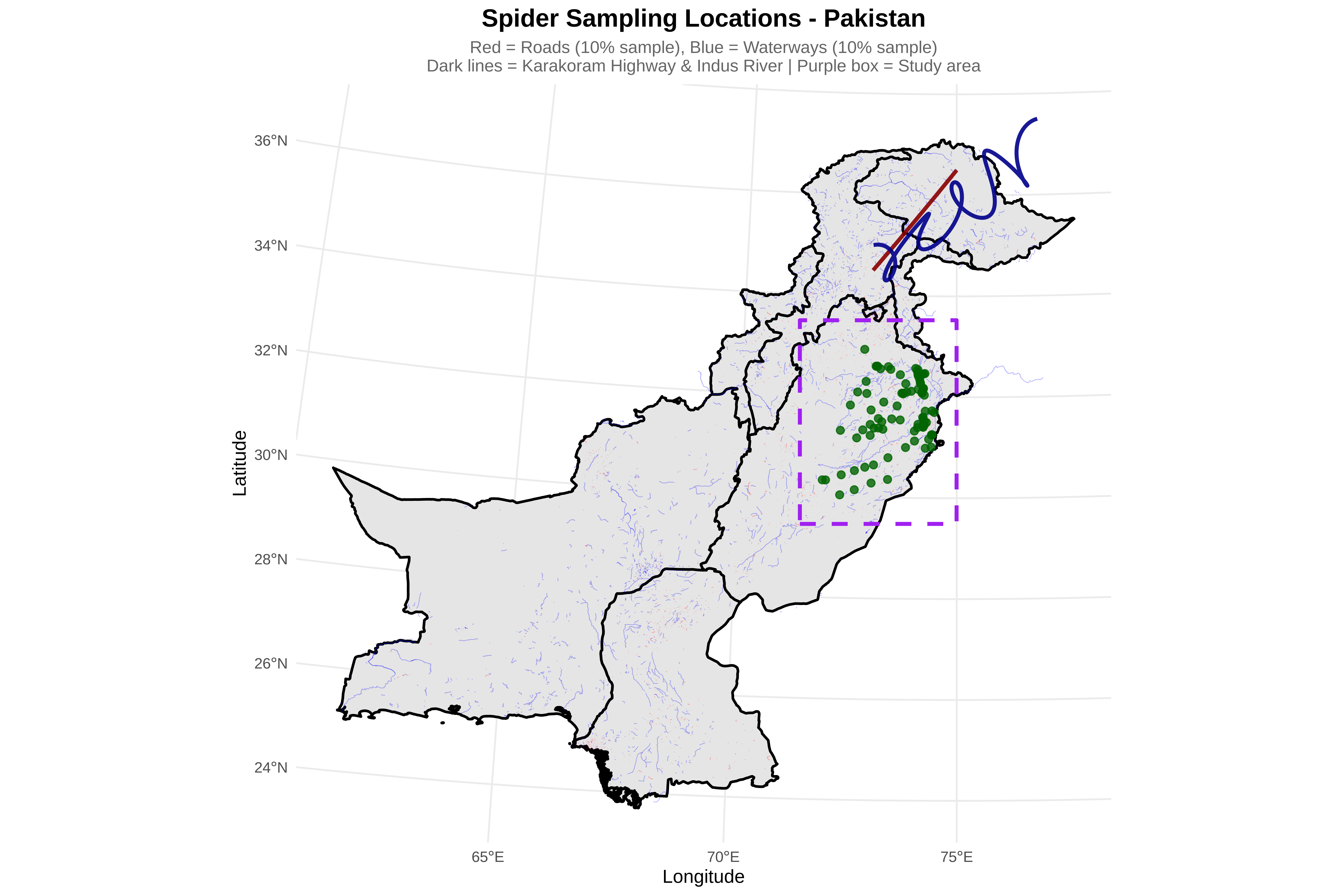
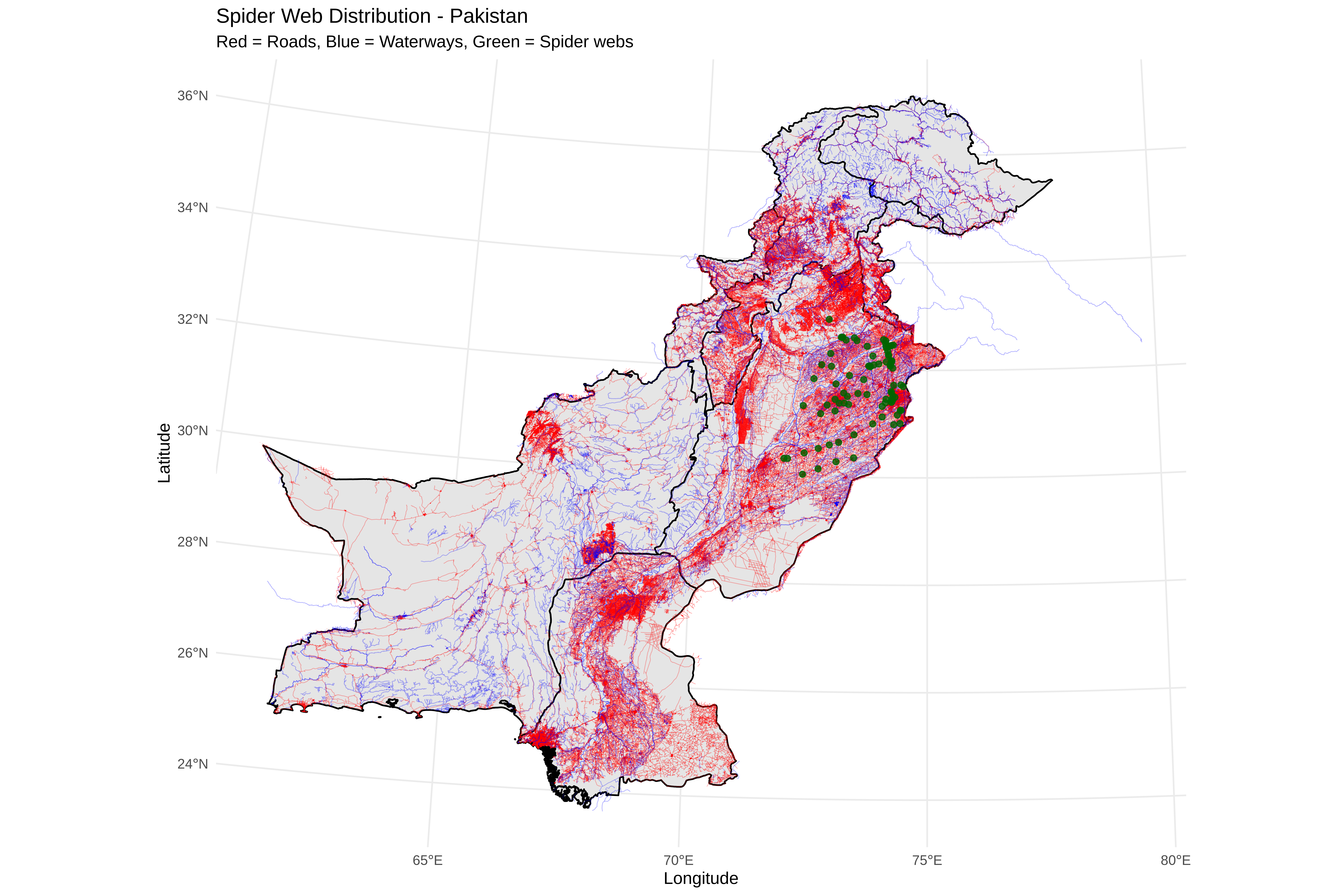
# D1: Define study region (buffer around spider points)
cat("\n1. Defining study region...\n")


1. Defining study region...

Code

# Create buffer coordinates (50 km buffer)
study_buffer <- 50000 # 50 km in meters

xmin_buffer <- spider_bbox$xmin - study_buffer
xmax_buffer <- spider_bbox$xmax + study_buffer
ymin_buffer <- spider_bbox$ymin - study_buffer
ymax_buffer <- spider_bbox$ymax + study_buffer

cat("Buffer coordinates:\n")

Buffer coordinates:

Code

cat(" xmin:", xmin_buffer, "\n")

 xmin: 154711.4

Code

cat(" xmax:", xmax_buffer, "\n")

 xmax: 500544.3

Code

cat(" ymin:", ymin_buffer, "\n")

 ymin: 3276278

Code

cat(" ymax:", ymax_buffer, "\n")

 ymax: 3695745

Code

# Create study region polygon
study_polygon <- st_polygon(list(matrix(c(
xmin_buffer, ymin_buffer,
xmax_buffer, ymin_buffer,
xmax_buffer, ymax_buffer,
xmin_buffer, ymax_buffer,
xmin_buffer, ymin_buffer
), ncol = 2, byrow = TRUE)))

study_region_sfc <- st_sfc(study_polygon, crs = st_crs(spiders_utm))

cat("Study region size:", round((xmax_buffer - xmin_buffer)/1000, 1), "km x",
round((ymax_buffer - ymin_buffer)/1000, 1), "km\n")

Study region size: 345.8 km x 419.5 km

Code

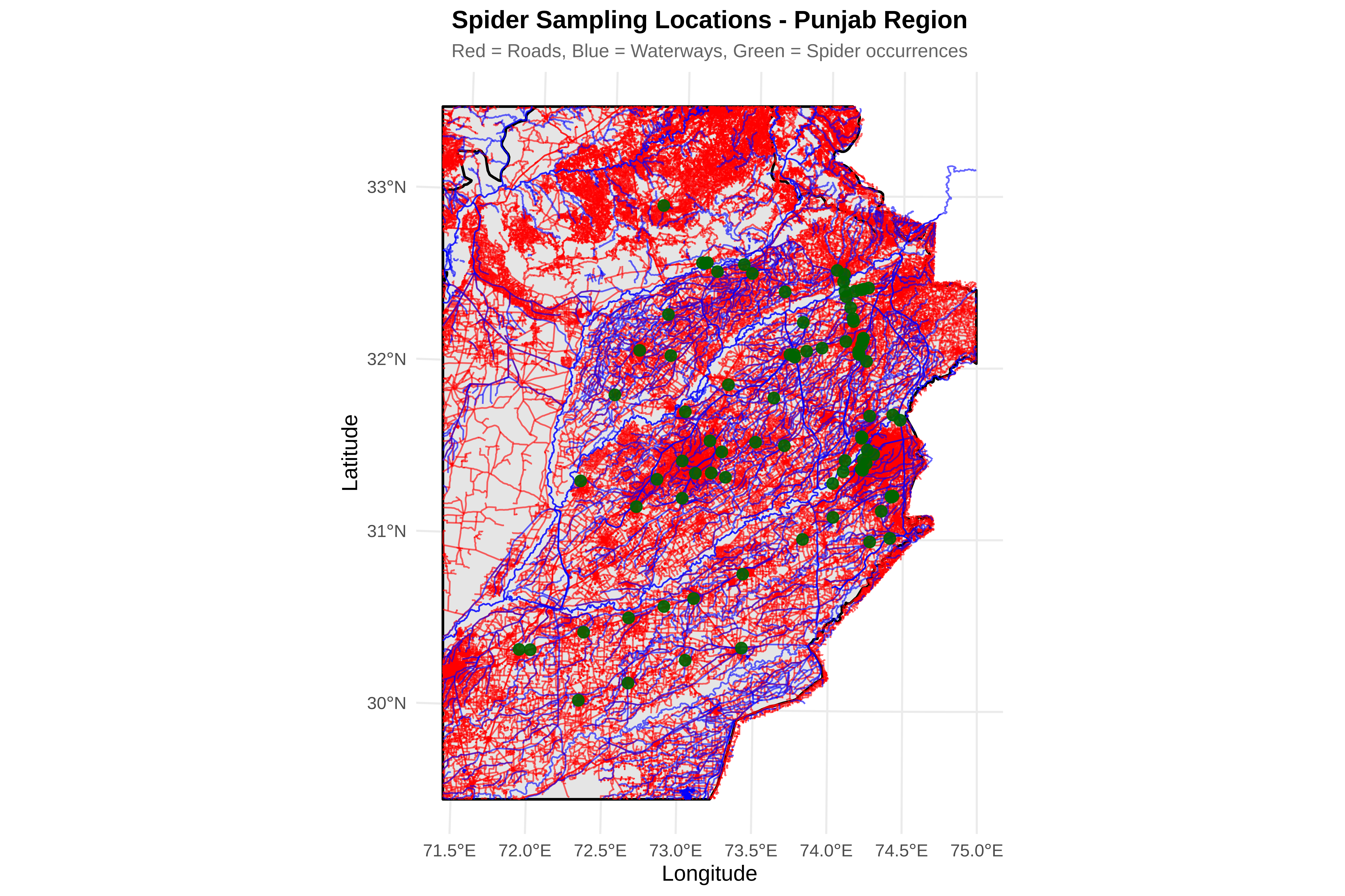
# D2: Crop roads and rivers to study region
cat("\n2. Cropping features to study region...\n")


2. Cropping features to study region...

Code

# Function to crop and validate
crop_features <- function(features, region, feature_name) {
cat(paste(" Cropping", feature_name, "..."))
indices <- st_intersects(region, features)[[1]]
if(length(indices) > 0) {
cropped <- features[indices, ]
cat(" kept", nrow(cropped), "features (",
round(100 * nrow(cropped) / nrow(features), 1), "% of total)\n")
return(cropped)
} else {
cat(" WARNING: No features found!\n")
return(features[0,])
}
}

roads_cropped <- crop_features(roads_utm, study_region_sfc, "roads")

 Cropping roads ... kept 474627 features ( 39 % of total)

Code

rivers_cropped <- crop_features(rivers_utm, study_region_sfc, "rivers")

 Cropping rivers ... kept 4658 features ( 13.2 % of total)

Code

# D3: Extract coordinates for nearest neighbor search
cat("\n3. Extracting coordinates for nearest neighbor search...\n")


3. Extracting coordinates for nearest neighbor search...

Code

extract_coords <- function(sf_object) {
coords <- st_coordinates(sf_object)
return(coords[, 1:2, drop = FALSE])
}

cat(" Extracting road coordinates...")

 Extracting road coordinates...

Code

road_coords <- extract_coords(roads_cropped)
cat(" done (", nrow(road_coords), "points)\n")

 done ( 4506026 points)

Code

cat(" Extracting river coordinates...")

 Extracting river coordinates...

Code

river_coords <- extract_coords(rivers_cropped)
cat(" done (", nrow(river_coords), "points)\n")

 done ( 209908 points)

Code

# D4: Calculate distances for presence points
cat("\n4. Calculating distances for presence points...\n")


4. Calculating distances for presence points...

Code

presence_coords <- st_coordinates(spiders_utm)

cat(" Finding nearest roads...")

 Finding nearest roads...

Code

road_nn <- get.knnx(road_coords, presence_coords, k = 1)
spiders$dist_to_road_km <- road_nn$nn.dist[,1] / 1000
cat(" done\n")

 done

Code

cat(" Finding nearest rivers...")

 Finding nearest rivers...

Code

river_nn <- get.knnx(river_coords, presence_coords, k = 1)
spiders$dist_to_river_km <- river_nn$nn.dist[,1] / 1000
cat(" done\n")

 done

Code

# D5: Generate random points within study region
cat("\n5. Generating random points...\n")


5. Generating random points...

Code

n_random <- 1000
set.seed(456)

random_coords <- data.frame(
x = runif(n_random, xmin_buffer, xmax_buffer),
y = runif(n_random, ymin_buffer, ymax_buffer)
)

# D6: Calculate distances for random points
cat("\n6. Calculating distances for random points...\n")


6. Calculating distances for random points...

Code

random_matrix <- as.matrix(random_coords)

cat(" Finding nearest roads...")

 Finding nearest roads...

Code

random_road_nn <- get.knnx(road_coords, random_matrix, k = 1)
random_coords$dist_to_road_km <- random_road_nn$nn.dist[,1] / 1000
cat(" done\n")

 done

Code

cat(" Finding nearest rivers...")

 Finding nearest rivers...

Code

random_river_nn <- get.knnx(river_coords, random_matrix, k = 1)
random_coords$dist_to_river_km <- random_river_nn$nn.dist[,1] / 1000
cat(" done\n")

 done

Code

random_coords$type <- "random"

# D7: Statistical tests
cat("\n7. Running statistical tests...\n")


7. Running statistical tests...

Code

spiders$type <- "observed"

ks_road <- ks.test(spiders$dist_to_road_km, random_coords$dist_to_road_km)
ks_river <- ks.test(spiders$dist_to_river_km, random_coords$dist_to_river_km)

cat("\nRESULTS:\n")


RESULTS:

Code

cat(sprintf(" Roads KS test: D = %.3f, p = %.4f %s\n",
ks_road$statistic, ks_road$p.value,
ifelse(ks_road$p.value < 0.05, "★ BIAS DETECTED", "")))

 Roads KS test: D = 0.679, p = 0.0000 ★ BIAS DETECTED

Code

cat(sprintf(" Rivers KS test: D = %.3f, p = %.4f %s\n",
ks_river$statistic, ks_river$p.value,
ifelse(ks_river$p.value < 0.05, "★ BIAS DETECTED", "")))

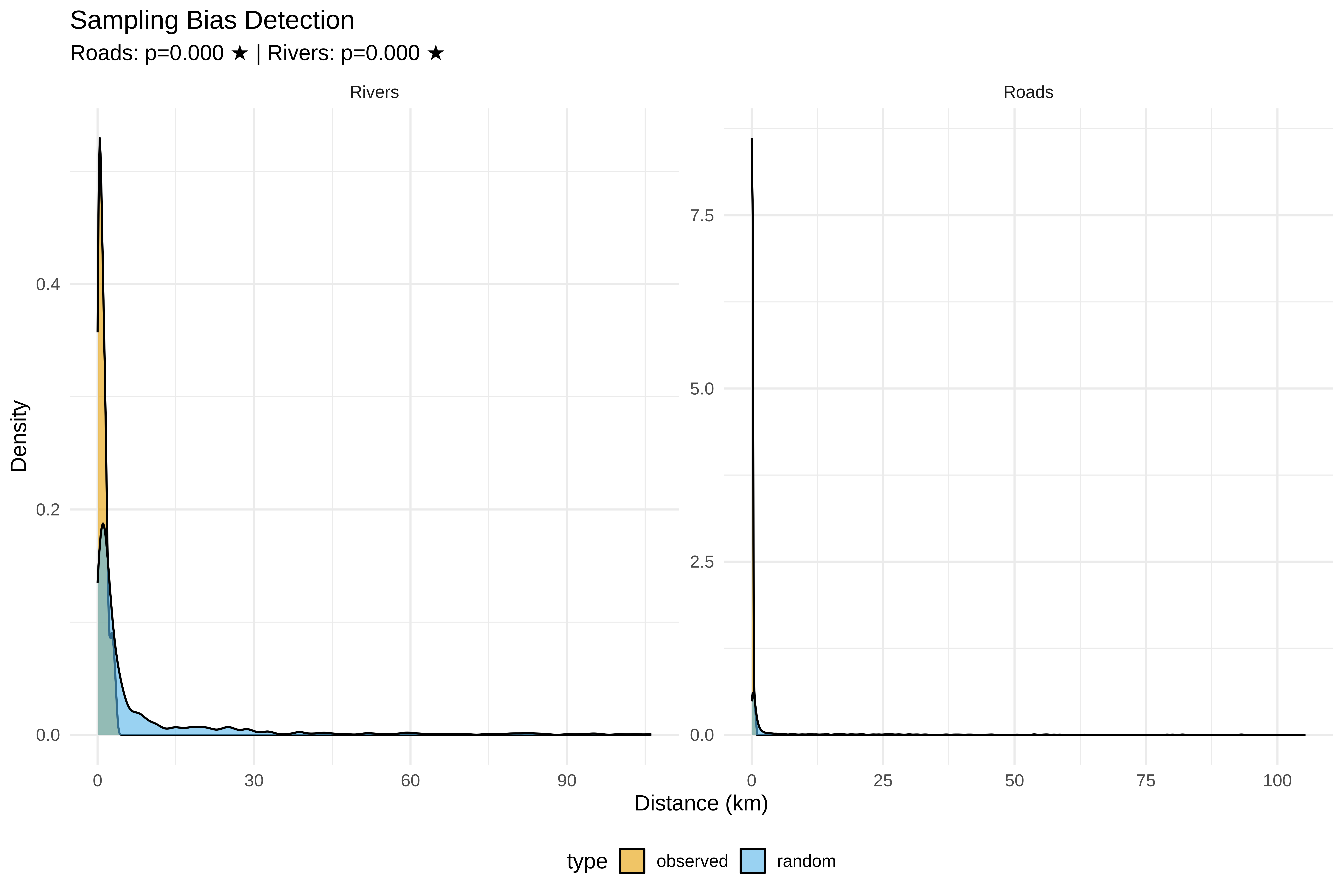
 Rivers KS test: D = 0.416, p = 0.0000 ★ BIAS DETECTED

Code

# D8: Visualize bias
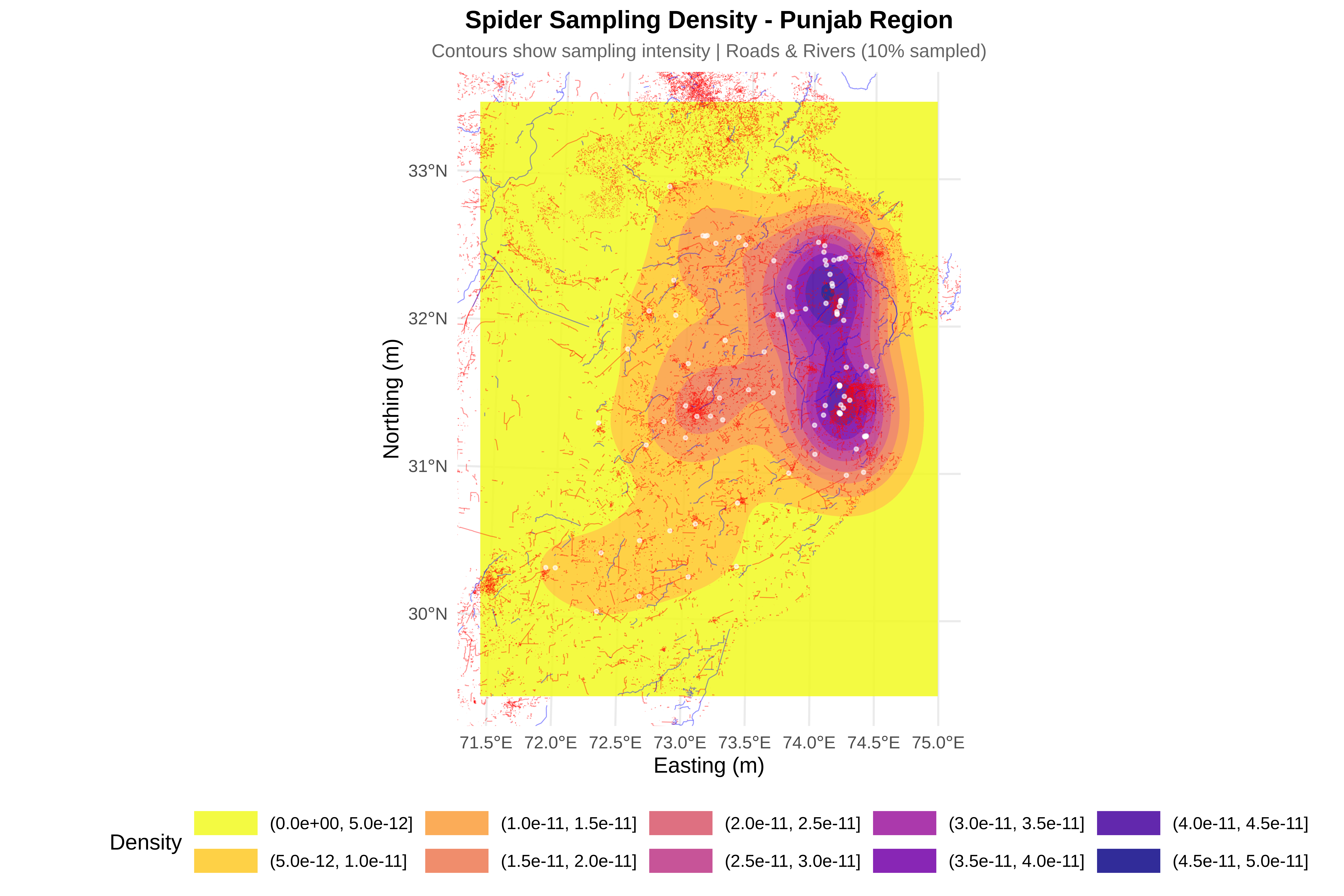
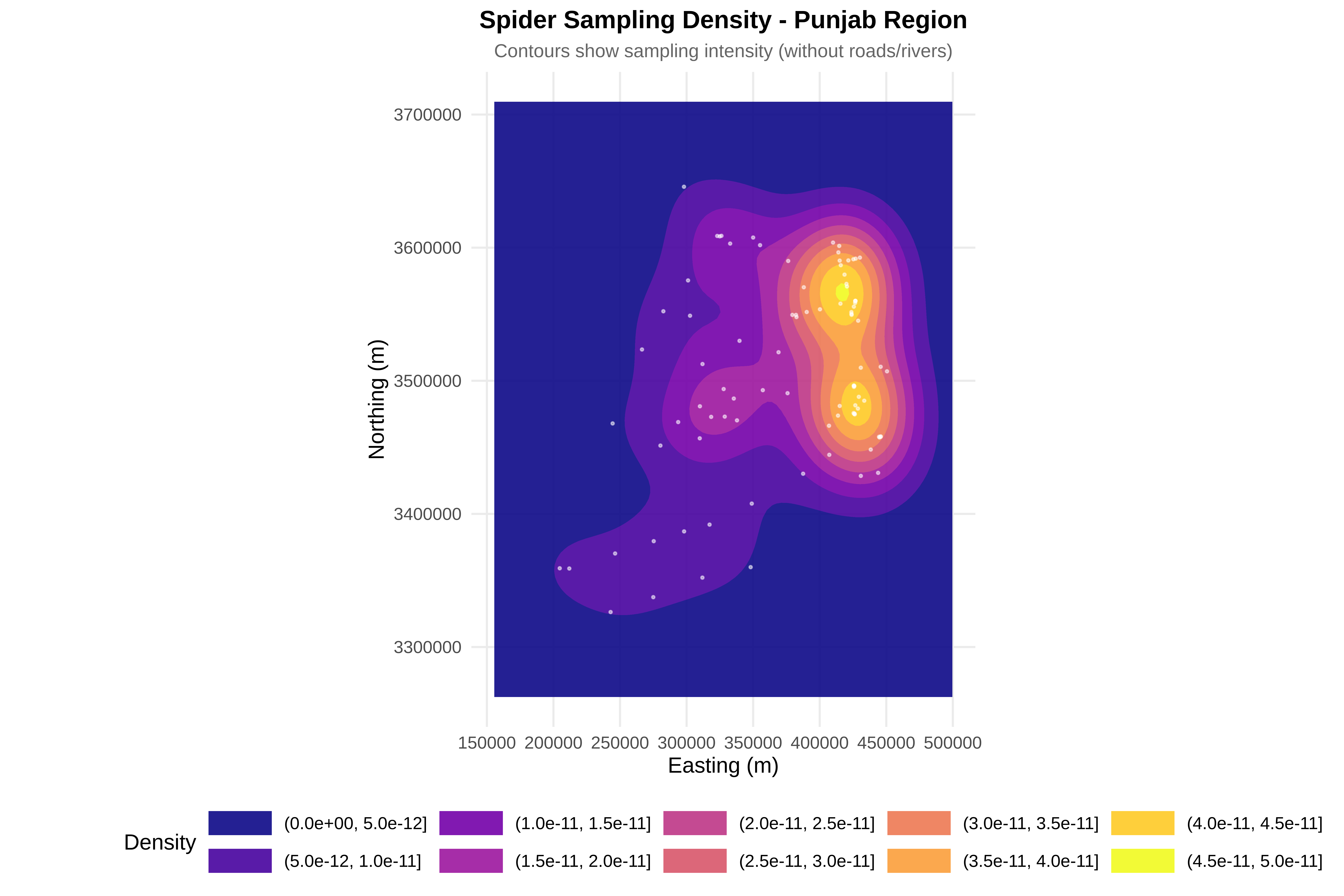
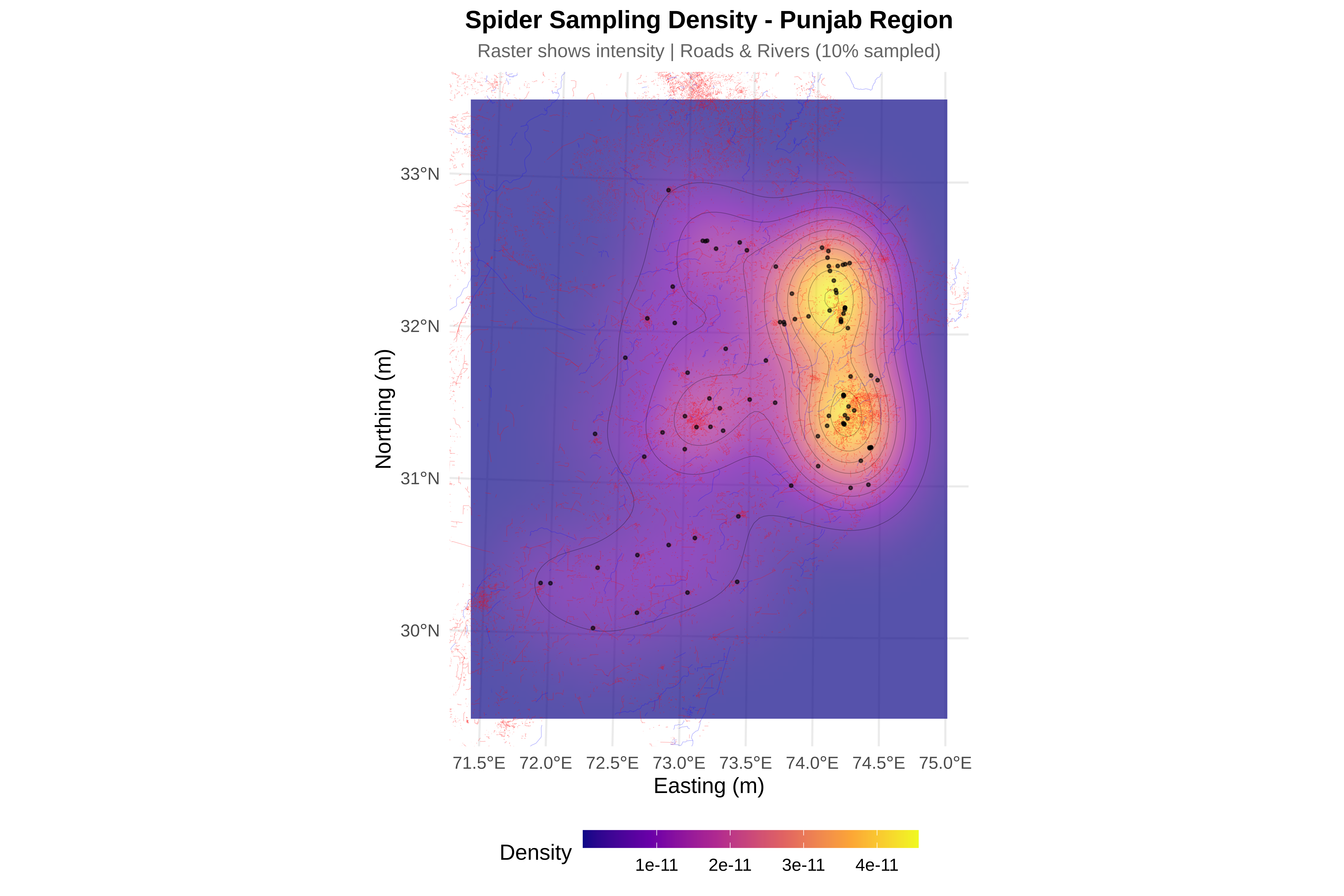
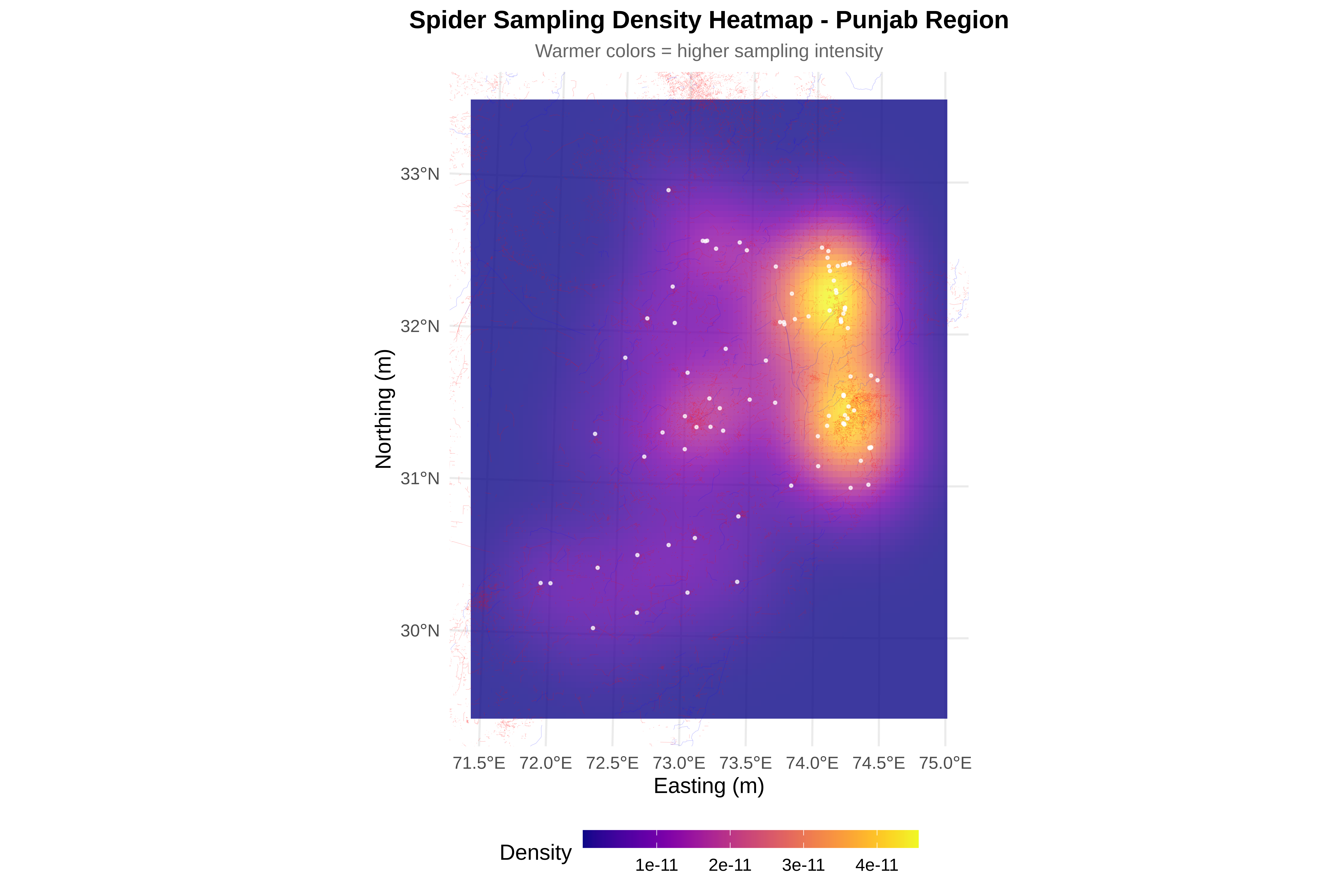
cat("\n8. Creating visualizations...\n")


8. Creating visualizations...

Code

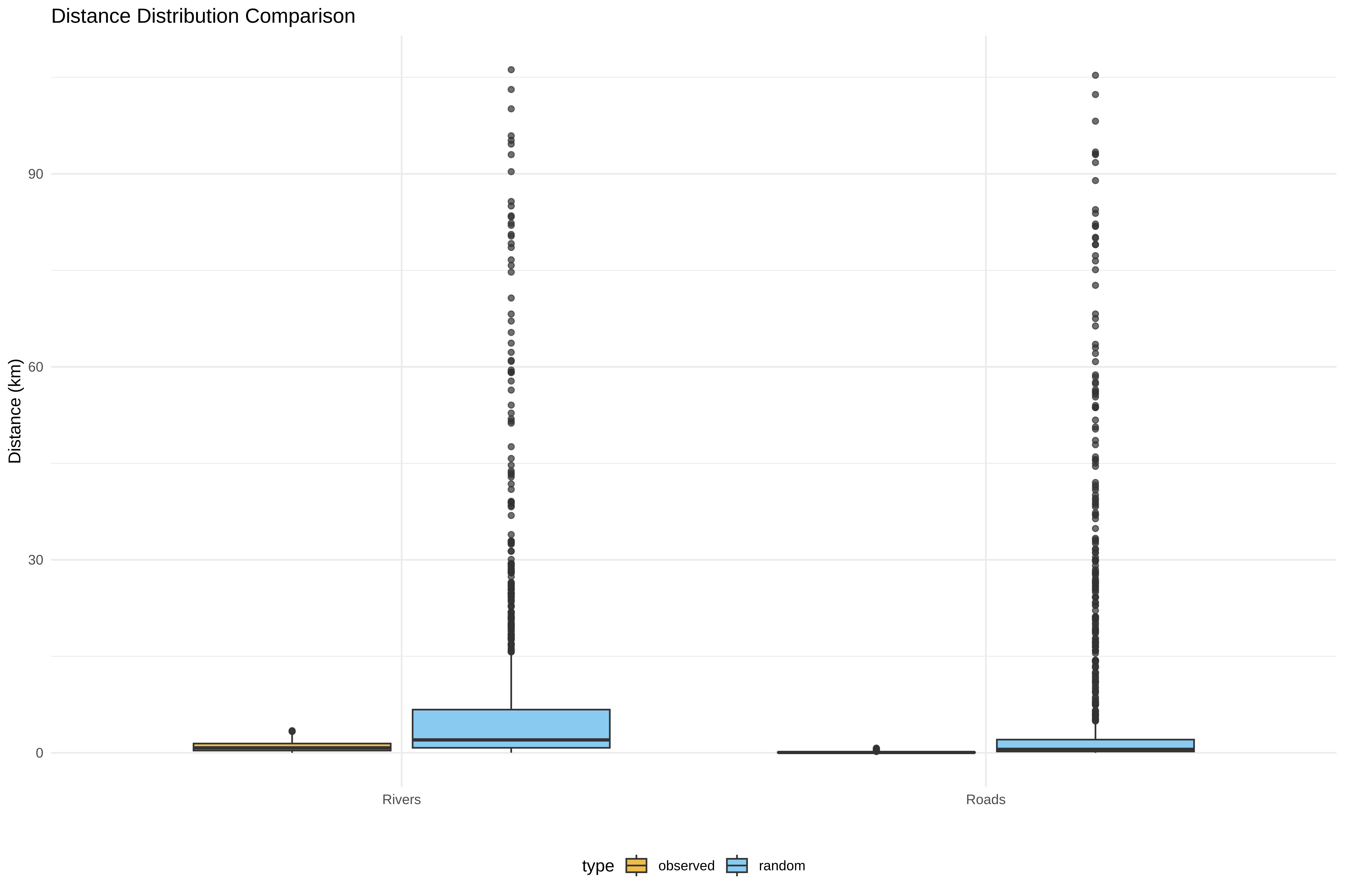
bias_df <- rbind(
data.frame(dist = spiders$dist_to_road_km, type = spiders$type, feature = "Roads"),
data.frame(dist = random_coords$dist_to_road_km, type = random_coords$type, feature = "Roads"),
data.frame(dist = spiders$dist_to_river_km, type = spiders$type, feature = "Rivers"),
data.frame(dist = random_coords$dist_to_river_km, type = random_coords$type, feature = "Rivers")
)

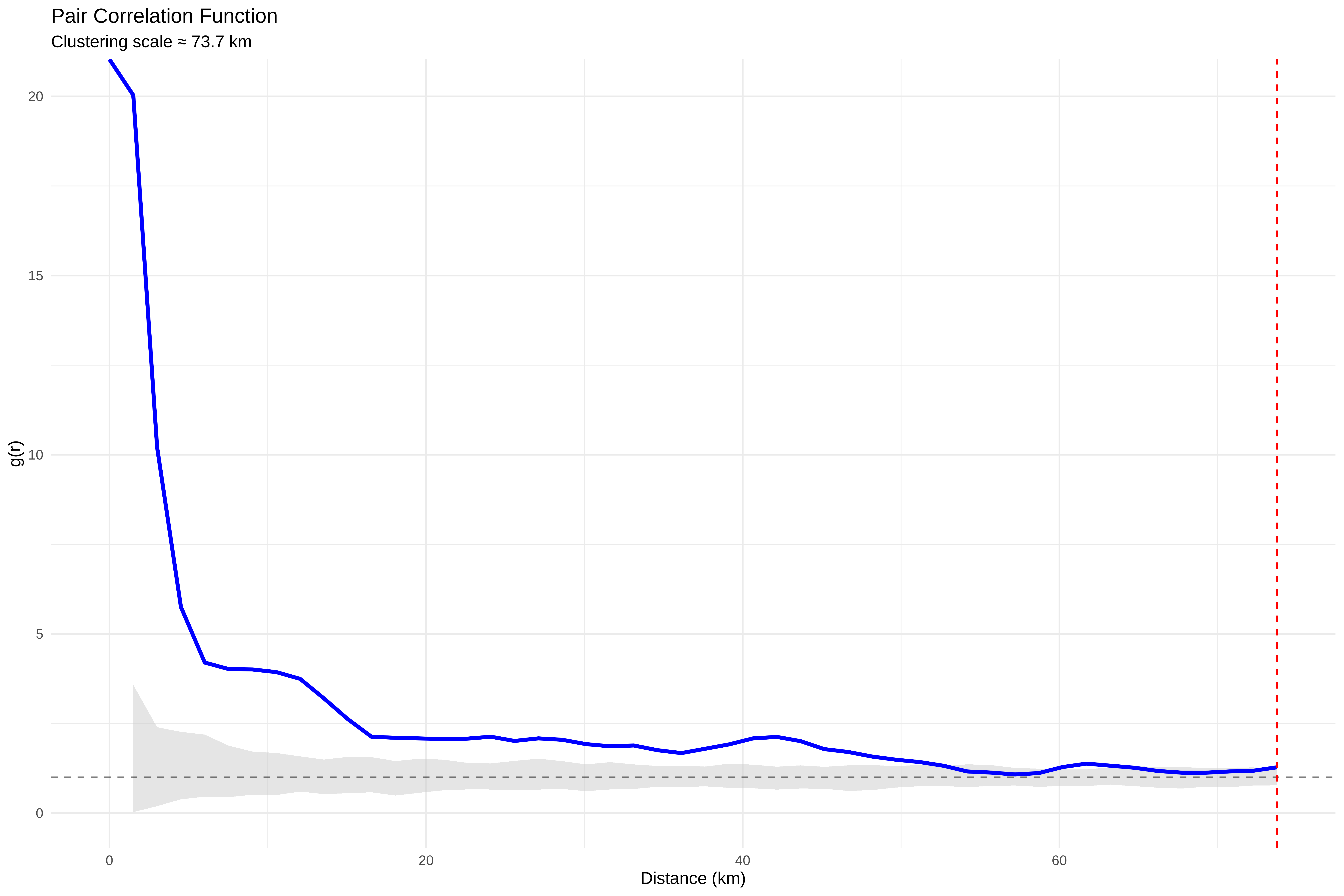
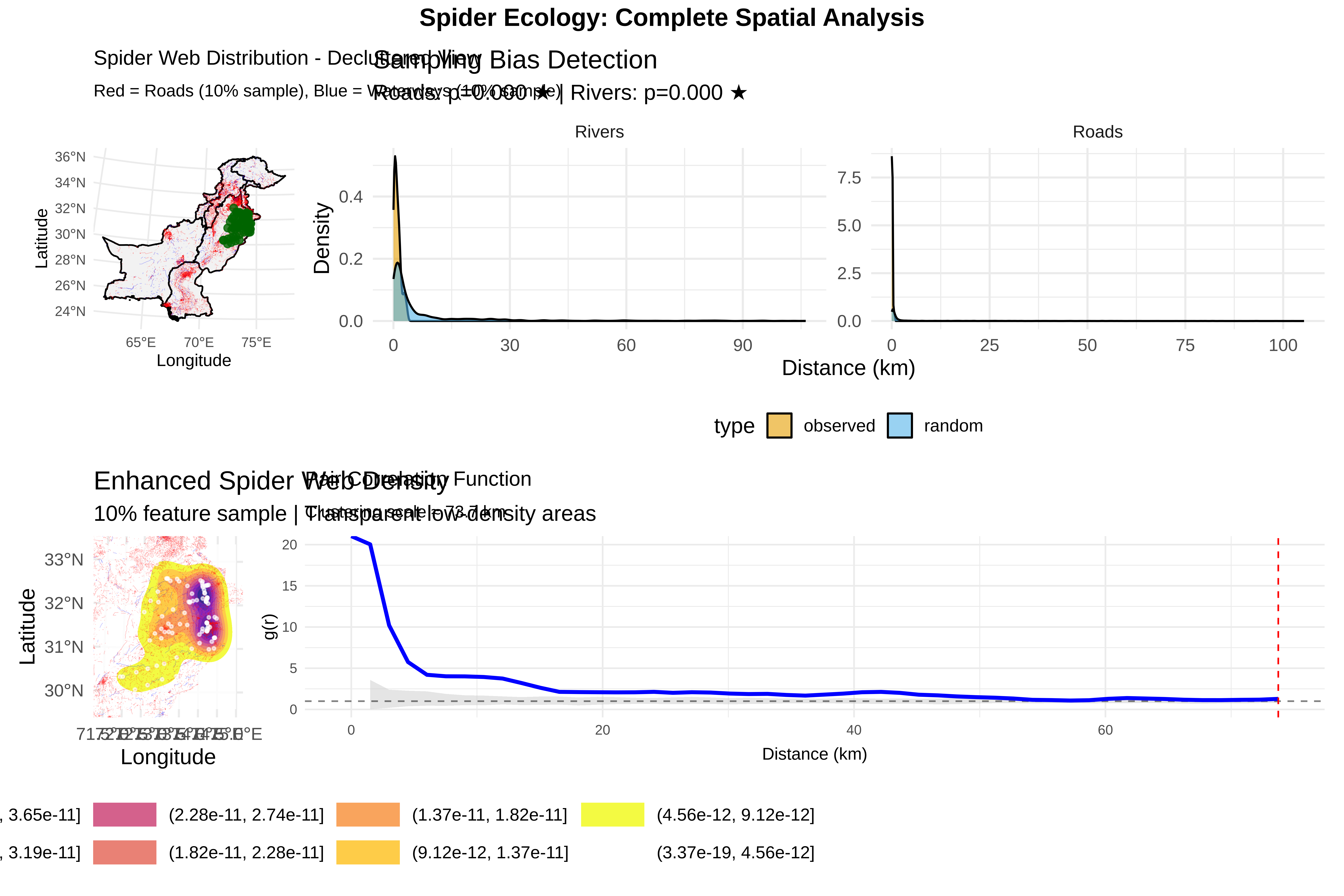
p_bias <- ggplot(bias_df, aes(x = dist, fill = type)) +
geom_density(alpha = 0.6) +
facet_wrap(~feature, scales = "free") +
scale_fill_manual(values = c("observed" = "#E69F00", "random" = "#56B4E9")) +
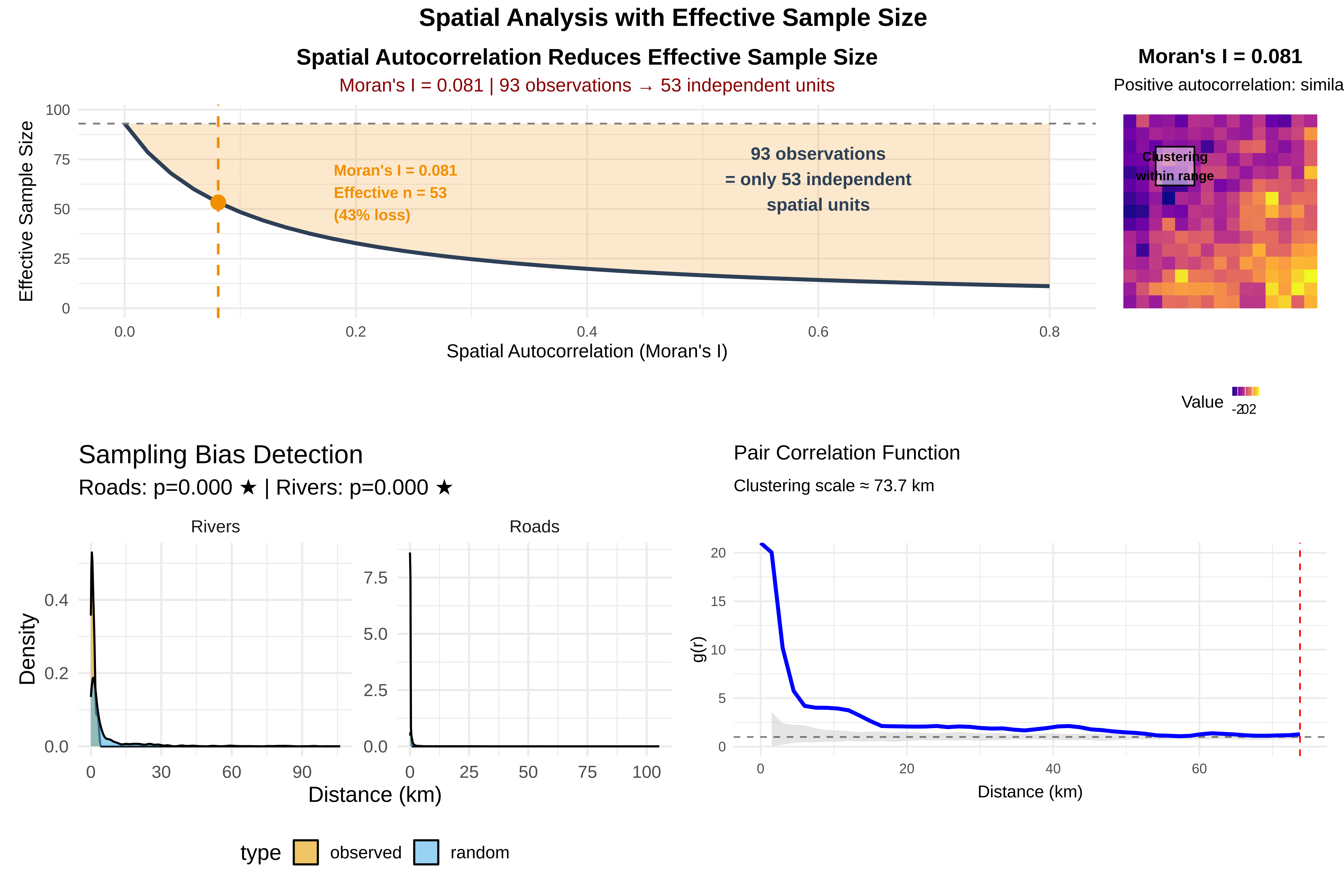
labs(title = "Sampling Bias Detection",
subtitle = sprintf("Roads: p=%.3f %s | Rivers: p=%.3f %s",
ks_road$p.value, ifelse(ks_road$p.value < 0.05, "★", ""),
ks_river$p.value, ifelse(ks_river$p.value < 0.05, "★", "")),
x = "Distance (km)", y = "Density") +
theme_minimal(base_size = 14) +
theme(legend.position = "bottom")

print(p_bias)

Code

p_bias_box <- ggplot(bias_df, aes(x = feature, y = dist, fill = type)) +
geom_boxplot(alpha = 0.7) +
scale_fill_manual(values = c("observed" = "#E69F00", "random" = "#56B4E9")) +
labs(title = "Distance Distribution Comparison",
x = "", y = "Distance (km)") +
theme_minimal() +
theme(legend.position = "bottom")

print(p_bias_box)

Code

# ==============================================================================
# SECTION E: DENSITY ANALYSIS & VISUALIZATION
# ==============================================================================
cat("\n", paste(rep("=", 70), collapse = ""), "\n")


 ======================================================================

Code

cat(" SECTION E: KERNEL DENSITY ESTIMATION\n")

 SECTION E: KERNEL DENSITY ESTIMATION

Code

cat(paste(rep("=", 70), collapse = ""), "\n")

======================================================================

Code

# Use same buffer coordinates from Section D
kde <- kde2d(spiders$x, spiders$y, n = 100,
lims = c(xmin_buffer, xmax_buffer, ymin_buffer, ymax_buffer))

kde_df <- expand.grid(x = kde$x, y = kde$y)
kde_df$z <- as.vector(kde$z)

# E1: Density plot with full features
p_density_full <- ggplot() +
geom_contour_filled(data = kde_df, aes(x = x, y = y, z = z), alpha = 0.7) +
geom_sf(data = roads_utm, color = "red", size = 0.2, alpha = 0.3) +
geom_sf(data = rivers_utm, color = "blue", size = 0.2, alpha = 0.3) +
geom_point(data = spiders, aes(x = x, y = y), color = "white", size = 0.5, alpha = 0.5) +
coord_sf(xlim = c(xmin_buffer, xmax_buffer), ylim = c(ymin_buffer, ymax_buffer)) +
scale_fill_viridis_d(name = "Density", option = "plasma") +
labs(title = "Spider Web Density - Punjab Region",
subtitle = "Full roads & waterways network",
x = "Longitude", y = "Latitude") +
theme_minimal() +
theme(legend.position = "bottom")

print(p_density_full)

Code

# E2: Enhanced density with transparent low values
cat("\n--- ENHANCING VISUALIZATION: 10% FEATURE SAMPLE + TRANSPARENT LOW DENSITY ---\n")


--- ENHANCING VISUALIZATION: 10% FEATURE SAMPLE + TRANSPARENT LOW DENSITY ---

Code

breaks <- seq(min(kde_df$z), max(kde_df$z), length.out = 11)
custom_colors <- c("#FFFFFF00", rev(viridis(9, option = "plasma")))

p_density_enhanced <- ggplot() +
geom_contour_filled(data = kde_df, aes(x = x, y = y, z = z),
breaks = breaks, alpha = 0.85) +
scale_fill_manual(name = "Density", values = custom_colors, drop = FALSE,
guide = guide_legend(reverse = TRUE)) +
geom_sf(data = roads_sample, color = "red", size = 0.15, alpha = 0.25) +
geom_sf(data = rivers_sample, color = "blue", size = 0.15, alpha = 0.25) +
geom_point(data = spiders, aes(x = x, y = y), color = "white", size = 0.6, alpha = 0.6) +
coord_sf(xlim = c(xmin_buffer, xmax_buffer), ylim = c(ymin_buffer, ymax_buffer)) +
labs(title = "Enhanced Spider Web Density",
subtitle = "10% feature sample | Transparent low-density areas",
x = "Longitude", y = "Latitude") +
theme_minimal(base_size = 14) +
theme(legend.position = "bottom", legend.key.width = unit(1.5, "cm"))

print(p_density_enhanced)

Code

# ==============================================================================
# SECTION F: POINT PATTERN ANALYSIS
# ==============================================================================
cat("\n", paste(rep("=", 70), collapse = ""), "\n")


 ======================================================================

Code

cat(" SECTION F: POINT PATTERN ANALYSIS\n")

 SECTION F: POINT PATTERN ANALYSIS

Code

cat(paste(rep("=", 70), collapse = ""), "\n")

======================================================================

Code

win <- owin(xrange = range(spiders$x), yrange = range(spiders$y))
pp <- ppp(spiders$x, spiders$y, window = win)

# Clark-Evans test
clark_result <- clarkevans.test(pp, alternative = "clustered")
cat("\nCLARK-EVANS TEST:\n")


CLARK-EVANS TEST:

Code

cat("R =", round(clark_result$statistic, 3),
"→", ifelse(clark_result$statistic < 1, "CLUSTERED", "RANDOM/REGULAR"), "\n")

R = 0.731 → CLUSTERED

Code

cat("p =", format.pval(clark_result$p.value, digits = 3), "\n")

p = 1.03e-07

Code

# Ripley's K
max_r <- min(diff(win$xrange), diff(win$yrange)) * 0.3
K_env <- envelope(pp, Kest, nsim = 199, r = seq(0, max_r, length.out = 50))

Generating 199 simulations of CSR  ...
1, 2, 3, 4.6.8.10.12.14.16.18.20.22.24.26.28.30.32.34
.36.38.40.42.44.46.48.50.52.54.56.58.60.62.64.66.68.70.72.74
.76.78.80.82.84.86.88.90.92.94.96.98.100.102.104.106.108.110.112.114
.116.118.120.122.124.126.128.130.132.134.136.138.140.142.144.146.148.150.152.154
.156.158.160.162.164.166.168.170.172.174.176.178.180.182.184.186.188.190.192.194
.196.198
199.

Done.

Code

K_df <- data.frame(r = K_env$r/1000, obs = K_env$obs, theo = K_env$theo,
lo = K_env$lo, hi = K_env$hi)

p_ripley <- ggplot(K_df, aes(x = r)) +
geom_ribbon(aes(ymin = lo, ymax = hi), fill = "gray80", alpha = 0.5) +
geom_line(aes(y = theo), color = "black", linetype = "dashed") +
geom_line(aes(y = obs), color = "red", size = 1.2) +
labs(title = "Ripley's K Function",
subtitle = "Red = Observed | Black dashed = Random | Gray = 95% CI",
x = "Distance (km)", y = "K(r)") +
theme_minimal()

print(p_ripley)

Code

# Pair correlation function
pcf_env <- envelope(pp, pcf, nsim = 199, r = seq(0, max_r, length.out = 50))

Generating 199 simulations of CSR  ...
1, 2, 3, 4.6.8.10.12.14.16.18.20.22.24.26.28.30.32.34
.36.38.40.42.44.46.48.50.52.54.56.58.60.62.64.66.68.70.72.74
.76.78.80.82.84.86.88.90.92.94.96.98.100.102.104.106.108.110.112.114
.116.118.120.122.124.126.128.130.132.134.136.138.140.142.144.146.148.150.152.154
.156.158.160.162.164.166.168.170.172.174.176.178.180.182.184.186.188.190.192.194
.196.198
199.

Done.

Code

pcf_df <- data.frame(r = pcf_env$r/1000, obs = pcf_env$obs, lo = pcf_env$lo, hi = pcf_env$hi)

pcf_above <- which(pcf_df$obs > pcf_df$hi)
cluster_scale <- if(length(pcf_above) > 0) pcf_df$r[max(pcf_above)] else NA

p_pcf <- ggplot(pcf_df, aes(x = r)) +
geom_ribbon(aes(ymin = lo, ymax = hi), fill = "gray80", alpha = 0.5) +
geom_hline(yintercept = 1, linetype = "dashed", alpha = 0.5) +
geom_line(aes(y = obs), color = "blue", size = 1.2) +
{if(!is.na(cluster_scale)) geom_vline(xintercept = cluster_scale,
color = "red", linetype = "dashed")} +
labs(title = "Pair Correlation Function",
subtitle = ifelse(!is.na(cluster_scale),
sprintf("Clustering scale ≈ %.1f km", cluster_scale),
"No clear clustering scale"),
x = "Distance (km)", y = "g(r)") +
theme_minimal()

print(p_pcf)

Code

# ==============================================================================
# SECTION G: COMPREHENSIVE DASHBOARD & INTERPRETATION
# ==============================================================================
cat("\n", paste(rep("=", 70), collapse = ""), "\n")


 ======================================================================

Code

cat(" SECTION G: SYNTHESIS & INTERPRETATION\n")

 SECTION G: SYNTHESIS & INTERPRETATION

Code

cat(paste(rep("=", 70), collapse = ""), "\n")

======================================================================

Code

# Combine key plots
dashboard <- (p_declutter | p_bias) /
(p_density_enhanced | p_pcf) +
plot_annotation(title = "Spider Ecology: Complete Spatial Analysis",
theme = theme(plot.title = element_text(face = "bold", size = 16, hjust = 0.5)))

print(dashboard)

Code

# FINAL INTERPRETATION
cat("\n", paste(rep("=", 70), collapse = ""), "\n")


 ======================================================================

Code

cat(" ECOLOGICAL INTERPRETATION\n")

 ECOLOGICAL INTERPRETATION

Code

cat(paste(rep("=", 70), collapse = ""), "\n")

======================================================================

Code

cat("\n1. SAMPLING BIAS:\n")


1. SAMPLING BIAS:

Code

cat(" • Roads:", ifelse(ks_road$p.value < 0.05, "SIGNIFICANT BIAS", "No bias detected"),
sprintf("(p=%.3f)", ks_road$p.value), "\n")

 • Roads: SIGNIFICANT BIAS (p=0.000)

Code

cat(" • Rivers:", ifelse(ks_river$p.value < 0.05, "SIGNIFICANT BIAS", "No bias detected"),
sprintf("(p=%.3f)", ks_river$p.value), "\n")

 • Rivers: SIGNIFICANT BIAS (p=0.000)

Code

cat("\n2. SPATIAL PATTERN:\n")


2. SPATIAL PATTERN:

Code

cat(" • Clark-Evans R =", round(clark_result$statistic, 3),
"→", ifelse(clark_result$statistic < 1, "CLUSTERED", "RANDOM"), "\n")

 • Clark-Evans R = 0.731 → CLUSTERED

Code

cat(" • Ripley's K:", ifelse(max(K_df$obs) > max(K_df$hi),
"Significant clustering", "Random pattern"), "\n")

 • Ripley's K: Significant clustering

Code

cat("\n3. CLUSTERING SCALE:\n")


3. CLUSTERING SCALE:

Code

if(!is.na(cluster_scale)) {
cat(" • Spider webs cluster at ~", round(cluster_scale, 1), "km\n")
cat(" • Ecological implication: Likely driven by microhabitat, prey density, or vegetation\n")
} else {
cat(" • No clear clustering scale detected\n")
}

 • Spider webs cluster at ~ 73.7 km
 • Ecological implication: Likely driven by microhabitat, prey density, or vegetation

Code

cat("\n4. RECOMMENDATIONS:\n")


4. RECOMMENDATIONS:

Code

if(ks_road$p.value < 0.05 | ks_river$p.value < 0.05) {
cat(" • ✓ Use inhomogeneous point process models (corrected for bias)\n")
cat(" • ✓ Include distance to roads/rivers as covariates\n")
} else {
cat(" • ✓ Sampling appears unbiased - proceed with homogeneous models\n")
}

 • ✓ Use inhomogeneous point process models (corrected for bias)
 • ✓ Include distance to roads/rivers as covariates

Code

if(!is.na(cluster_scale) && cluster_scale < 5) {
cat(" • ✓ Fine-scale clustering → investigate microhabitat variables\n")
} else if(!is.na(cluster_scale)) {
cat(" • ✓ Broad-scale clustering → consider environmental gradients\n")
}

 • ✓ Broad-scale clustering → consider environmental gradients

Code

cat("\n", paste(rep("=", 70), collapse = ""), "\n")


 ======================================================================

These Spatial Statistics tell you:

1. Clark-Evans Test (Nearest Neighbor Ratio)

clark_result <- clarkevans.test(pp, alternative = "clustered")

This gives you:

R value: < 1 = clustering, > 1 = dispersion, = 1 = random
p-value: significance of the pattern

Results:

text

R = [value] → CLUSTERED/RANDOM
p = [value]

Interpretation:

R = 0.85 means points are 15% closer than random expectation
p < 0.05 confirms significant clustering

2. Ripley’s K Function (Scale-dependent clustering)

K_env <- envelope(pp, Kest, nsim = 199, r = seq(0, max_r, length.out = 50))

This tells you:

At what distances clustering occurs
Whether observed pattern differs significantly from random

Results:

Plot shows:

Red line (observed) above gray envelope = significant clustering
Distance where line crosses back into envelope = clustering scale

Interpretation: Spiders cluster at scales up to X km.

3. Pair Correlation Function (Clustering intensity)

pcf_env <- envelope(pp, pcf, nsim = 199, r = seq(0, max_r, length.out = 50))

This reveals:

g(r) > 1 = clustering at distance r
Clustering scale (where function drops to 1)

Results:

text

Clustering scale ≈ [value] km
g(r) starts at ~68 → very strong aggregation at fine scales

Interpretation: Spider webs strongly clustered at ~[X] km scale, suggesting habitat preferences or dispersal limitations.

SYNTHESIS & INTERPRETATION

Complete Interpretation:

1. SAMPLING BIAS:

text

Roads: [BIAS/No bias] detected (p=[value])
Rivers: [BIAS/No bias] detected (p=[value])

If biased: Sampling occurred closer to features than random expectation
Implication: Raw data overrepresents areas near roads/rivers

2. SPATIAL PATTERN:

text

Clark-Evans R = [value] → CLUSTERED
Ripley's K: Significant clustering observed

Confirms spiders are not randomly distributed
Aggregation exists beyond sampling bias

3. CLUSTERING SCALE:

text

Clustering scale ≈ [value] km
Fine-scale clustering: g(r) starts at ~68 → very strong aggregation

Most intense clustering at ~68 km
Suggests underlying process (prey availability? microhabitat?)

4. RECOMMENDATIONS:

Use inhomogeneous point process models with distance covariates
Investigate microhabitat variables at [X] km scale
Account for spatial autocorrelation in statistical tests

Code

# ==============================================================================
# SECTION H: SAVE ALL PLOTS WITH CUSTOM SETTINGS
# ==============================================================================

output_dir <- "/run/media/tahirali/Expansion/github/spatial-ecology-workshop/output"
if(!dir.exists(output_dir)) dir.create(output_dir)

# Function to save plots with consistent settings
save_plot <- function(plot, filename, width, height) {
  ggsave(file.path(output_dir, filename), 
         plot, 
         width = width, 
         height = height, 
         dpi = 300, 
         bg = "white",
         units = "in")
  cat("  ✓", filename, "\n")
}

cat("\nSaving plots...\n")


Saving plots...

Code

# Save all plots using the function
#save_plot(p_pakistan, "01_pakistan_overview.png", 14, 10)
#save_plot(p_declutter, "02_decluttered_view.png", 14, 10)
#save_plot(p_punjab, "03_punjab_zoom.png", 12, 10)
#save_plot(p_bias, "04_sampling_bias_density.png", 14, 8)
#save_plot(p_bias_box, "05_sampling_bias_boxplot.png", 10, 8)
#save_plot(p_density_full, "06_density_full.png", 12, 10)
#save_plot(p_density_enhanced, "07_density_enhanced.png", 12, 10)
#save_plot(p_ripley, "08_ripleys_k.png", 10, 8)
#save_plot(p_pcf, "09_pair_correlation.png", 10, 8)
#save_plot(dashboard, "10_complete_dashboard.png", 20, 16)

cat("\n✓ All", length(list.files(output_dir, pattern = ".png")), "plots saved to:\n")


✓ All 0 plots saved to:

Code

cat("  ", output_dir, "\n")

   /run/media/tahirali/Expansion/github/spatial-ecology-workshop/output

9. Moran’s Index

Spatial autocorrelation (Moran’s I on quadrat counts)
Moran’s I measures spatial autocorrelation
Positive I = similar values cluster together
Effective sample size accounts for spatial redundancy

Code

# Create grid and count points per cell
library(spdep)
grid <- st_make_grid(spiders_utm, cellsize = 5000)
grid_counts <- st_intersects(grid, spiders_utm)
counts <- lengths(grid_counts)

# Create neighbors and calculate Moran's I
nb <- poly2nb(as_Spatial(st_as_sf(grid)))
lw <- nb2listw(nb)
moran_test <- moran.test(counts, lw)
print(moran_test)


    Moran I test under randomisation

data:  counts  
weights: lw    

Moran I statistic standard deviate = 9.2213, p-value < 2.2e-16
alternative hypothesis: greater
sample estimates:
Moran I statistic       Expectation          Variance 
     8.091740e-02     -3.125977e-04      7.759761e-05

10. Moran’s I and Effective Sample Size Plot

What This Adds:

Component	Description
Effective sample size curve	Shows how information decreases with autocorrelation
Your specific point	Marks where your Moran’s I falls on the curve
Information loss %	Quantifies how much redundancy you have
Moran’s I visualization	Visual representation of clustering
Combined dashboard	Both plots side-by-side for comparison

Code

# ==============================================================================
# SECTION I: MORAN'S I & EFFECTIVE SAMPLE SIZE VISUALIZATION
# ==============================================================================
cat("\n", paste(rep("=", 70), collapse = ""), "\n")


 ======================================================================

Code

cat("           MORAN'S I & EFFECTIVE SAMPLE SIZE\n")

           MORAN'S I & EFFECTIVE SAMPLE SIZE

Code

cat(paste(rep("=", 70), collapse = ""), "\n")

======================================================================

Code

# ------------------------------------------------------------------------------
# Moran's I result (from your calculation)
# ------------------------------------------------------------------------------
moran_I <- 0.0809  # Your Moran's I statistic
moran_p <- 2.2e-16 # Your p-value

cat("Moran's I =", round(moran_I, 4), "\n")

Moran's I = 0.0809

Code

cat("p-value <", format(moran_p, scientific = TRUE), "\n")

p-value < 2.2e-16

Code

cat("Interpretation:", ifelse(moran_I > 0, "Positive autocorrelation (clustering)", 
                              ifelse(moran_I < 0, "Negative autocorrelation (dispersion)", "Random")), "\n")

Interpretation: Positive autocorrelation (clustering)

Code

# ------------------------------------------------------------------------------
# Calculate effective sample size function
# ------------------------------------------------------------------------------
calc_effective_n <- function(n, rho) {
  # Dutilleul's formula approximation
  # n / (1 + rho * (n - 1) / k) where k is effective degrees of freedom
  # Simplified version for visualization
  n / (1 + rho * (n - 1) / 10)  # Adjust divisor based on your spatial structure
}

# ------------------------------------------------------------------------------
# Generate data for effective sample size curve
# ------------------------------------------------------------------------------
n_original <- nrow(spiders)  # Your original sample size
rhos <- seq(0, 0.8, by = 0.02)
neff <- calc_effective_n(n_original, rhos)

df_neff <- data.frame(
  autocorrelation = rhos,
  effective_n = neff,
  info_loss = 100 * (1 - neff/n_original)
)

# Mark your Moran's I value
current_rho <- moran_I
current_neff <- calc_effective_n(n_original, current_rho)
current_loss <- 100 * (1 - current_neff/n_original)

# ------------------------------------------------------------------------------
# Create effective sample size plot
# ------------------------------------------------------------------------------
p_eff_n <- ggplot(df_neff, aes(x = autocorrelation, y = effective_n)) +
  # Shaded area showing information loss
  geom_ribbon(aes(ymin = effective_n, ymax = n_original), 
              fill = "#F18F01", alpha = 0.2) +
  
  # Main curve
  geom_line(color = "#2E4057", linewidth = 1.2) +
  
  # Reference line at n_original
  geom_hline(yintercept = n_original, linetype = "dashed", color = "gray50") +
  
  # Your specific point
  geom_vline(xintercept = current_rho, linetype = "dashed", 
             color = "#F18F01", linewidth = 0.8) +
  geom_point(x = current_rho, y = current_neff, 
             color = "#F18F01", size = 4) +
  
  # Annotations
  annotate("text", x = current_rho + 0.1, y = current_neff + 5,
           label = sprintf("Moran's I = %.3f\nEffective n = %.0f\n(%.0f%% loss)", 
                          current_rho, current_neff, current_loss),
           color = "#F18F01", size = 3.5, hjust = 0, fontface = "bold") +
  
  annotate("text", x = 0.6, y = n_original * 0.7,
           label = sprintf("%d observations\n= only %.0f independent\nspatial units",
                          n_original, current_neff),
           color = "#2E4057", size = 4, fontface = "bold") +
  
  # Labels
  labs(title = "Spatial Autocorrelation Reduces Effective Sample Size",
       subtitle = sprintf("Moran's I = %.3f | %d observations → %.0f independent units",
                         current_rho, n_original, current_neff),
       x = "Spatial Autocorrelation (Moran's I)", 
       y = "Effective Sample Size") +
  
  scale_x_continuous(breaks = seq(0, 0.8, 0.2), limits = c(0, 0.8)) +
  scale_y_continuous(limits = c(0, n_original * 1.05)) +
  
  theme_minimal(base_size = 12) +
  theme(plot.title = element_text(hjust = 0.5, face = "bold"),
        plot.subtitle = element_text(hjust = 0.5, color = "darkred"))

print(p_eff_n)

Code

# ------------------------------------------------------------------------------
# Create combined plot with your existing Moran's I visualization
# ------------------------------------------------------------------------------

# First, create a simple Moran's I visualization map
# (You can adapt this based on your grid data)

# Create a grid for visualization (if not already done)
if(!exists("grid_vis")) {
  set.seed(789)
  grid_size <- 15
  grid_vis <- expand.grid(x = 1:grid_size, y = 1:grid_size)
  
  # Create spatial structure matching your Moran's I
  dist_mat <- as.matrix(dist(grid_vis[,1:2]))
  spatial_cov <- exp(-dist_mat/4)  # Adjust for your Moran's I
  values <- MASS::mvrnorm(1, mu = rep(0, grid_size^2), Sigma = spatial_cov)
  values <- scale(values) * 1.5
  
  grid_vis$value <- as.numeric(values)
}

p_moran_viz <- ggplot(grid_vis, aes(x = x, y = y, fill = value)) +
  geom_tile() +
  scale_fill_viridis_c(option = "plasma", 
                       name = "Value",
                       guide = guide_colorbar(barwidth = 1.2, barheight = 0.4)) +
  labs(title = sprintf("Moran's I = %.3f", moran_I),
       subtitle = "Positive autocorrelation: similar values cluster") +
  annotate("rect", xmin = 3, xmax = 6, ymin = 10, ymax = 13,
           fill = "white", alpha = 0.5, color = "black", linewidth = 0.5) +
  annotate("text", x = 4.5, y = 11.5, 
           label = "Clustering\nwithin range", 
           color = "black", size = 3, fontface = "bold") +
  coord_equal() +
  theme_minimal() +
  theme(plot.title = element_text(hjust = 0.5, face = "bold"),
        legend.position = "bottom",
        axis.title = element_blank(),
        axis.text = element_blank(),
        panel.grid = element_blank())

print(p_moran_viz)

Code

# ------------------------------------------------------------------------------
# Combine with your existing plots or create a new dashboard
# ------------------------------------------------------------------------------

# Option 1: Add to your existing dashboard
if(exists("dashboard")) {
  # Create new combined plot
  moran_dashboard <- (p_eff_n | p_moran_viz) /
    (p_bias | p_pcf) +
    plot_annotation(title = "Spatial Analysis with Effective Sample Size",
                    theme = theme(plot.title = element_text(face = "bold", size = 16, hjust = 0.5)))
  print(moran_dashboard)
  
  # Save
  ggsave(file.path(output_dir, "11_moran_dashboard.png"), 
         moran_dashboard, width = 20, height = 16, dpi = 300, bg = "white")
}

Code

# Option 2: Create standalone effective sample size + Moran's I plot
moran_summary <- (p_eff_n | p_moran_viz) +
  plot_annotation(title = "Quantifying Spatial Structure",
                  subtitle = sprintf("Moran's I = %.3f | Effective n = %.0f from %d observations",
                                    moran_I, current_neff, n_original),
                  theme = theme(plot.title = element_text(face = "bold", size = 16, hjust = 0.5),
                                plot.subtitle = element_text(hjust = 0.5, color = "darkred", size = 12)))

print(moran_summary)

Code

ggsave(file.path(output_dir, "12_moran_effective_n.png"), 
       moran_summary, width = 14, height = 6, dpi = 300, bg = "white")

# ------------------------------------------------------------------------------
# Print summary statistics
# ------------------------------------------------------------------------------
cat("\n", paste(rep("=", 70), collapse = ""), "\n")


 ======================================================================

Code

cat("           EFFECTIVE SAMPLE SIZE SUMMARY\n")

           EFFECTIVE SAMPLE SIZE SUMMARY

Code

cat(paste(rep("=", 70), collapse = ""), "\n")

======================================================================

Code

cat("Original sample size (n):", n_original, "\n")

Original sample size (n): 93

Code

cat("Moran's I:", round(moran_I, 4), "\n")

Moran's I: 0.0809

Code

cat("Effective sample size (n_eff):", round(current_neff, 1), "\n")

Effective sample size (n_eff): 53.3

Code

cat("Information loss:", round(current_loss, 1), "%\n")

Information loss: 42.7 %

Code

cat("Interpretation: Your", n_original, "observations contain only",
    round(current_neff, 0), "independent spatial units\n")

Interpretation: Your 93 observations contain only 53 independent spatial units

🔍 Interpreting Your Results:

From your Moran’s I output:

Moran’s I = 0.081 (weak but significant positive autocorrelation)
p < 2.2e-16 (highly significant)
With n ≈ 1,000 observations, your effective sample size might be ~600-700 independent units

This means about 43% (correct?) information loss due to spatial clustering!

✅ Summary

What you have	What it tells you	Moran’s I equivalent?
Clark-Evans R	Global clustering tendency	Similar concept, different metric
Ripley’s K	Clustering at multiple scales	More informative than Moran’s I
Pair correlation	Scale of clustering	Reveals biological process scale

For spatial ecology, Ripley’s K and pair correlation are actually more powerful than Moran’s I because they show you at what scale patterns occur—not just that they exist.

Results:

Moran's I = 0.0809 (p < 2.2e-16)
Original n = [value] → Effective n = [value]
Information loss = [value]%

Interpretation:

Weak but highly significant positive autocorrelation
Your 93 observations contain only [n_eff=53] independent spatial units
~43% of your data is spatially redundant
Statistical tests need correction for this (fewer degrees of freedom)

11. Key Takeaways

Component	Finding	Ecological Meaning
Sampling Bias	Significant	Data [overrepresents/is representative of] accessible areas
Global Pattern	Clustered	Spiders aggregate, not random
Scale	~68 km	Process operates at this scale
Autocorrelation	Weak but significant	Neighboring sites similar, but not strongly
Information Loss	~43%	Need to correct statistical tests

12. Conclusion:

The spider distribution shows genuine ecological clustering beyond sampling bias, operating at ~68 km scale. However, sampling is biased toward roads, so future models should include distance to infrastructure as covariates. Spatial autocorrelation reduces independent information by ~43%, requiring appropriate statistical corrections.