Session 4: Multivariate & Dimensionality Reduction

Advanced Spatial Ecology & Species Distribution Modeling

Author

Dr Tahir Ali | AG de Meaux | TRR341 Ecological Genomics | University of Cologne

Code
# Setup chunk - runs before everything else
knitr::opts_chunk$set(echo = TRUE, message = FALSE, warning = FALSE)

# Create output directory if it doesn't exist
output_dir <- "/run/media/tahirali/Expansion/github/spatial-ecology-workshop/output/Session_4"
dir.create(output_dir, showWarnings = FALSE, recursive = TRUE)

Session Overview

Learning Outcomes:

  • Interpret PCA axes as ecological gradients

  • Read loadings (what “defines” each gradient)

  • Use UMAP/t-SNE for visualization (not inference)

  • Build climate niche space plots

🔗 Connection to Session 3: In Session 3 we diagnosed collinearity (VIF > 10 for several temperature variables) and used regularization to handle it. Here we take a different approach — instead of selecting or dropping variables, PCA creates new uncorrelated axes that capture the major environmental gradients. We then visualize the species’ climate niche in this reduced space.

Code
# ==============================================================================
# STEP 1: LOAD REQUIRED PACKAGES
# ==============================================================================
# Packages carried over from Session 3 + new ones for dimensionality reduction

library(ggplot2)      # Professional-looking plots
library(dplyr)        # Data manipulation
library(tidyr)        # Reshaping data (long vs wide formats)
library(terra)        # Working with raster data (climate TIFFs)
library(sf)           # Working with spatial vector data (shapefiles)
library(viridis)      # Color-blind friendly color schemes
library(patchwork)    # Combining multiple plots into one
library(MASS)         # For 2D kernel density estimation (kde2d)
library(uwot)         # For UMAP (Uniform Manifold Approximation and Projection)

# Set seed for reproducibility
set.seed(123)

1. LOAD AND PREPARE DATA (Same Pipeline as Session 3)

Code
# ==============================================================================
# STEP 2: DEFINE FILE PATHS
# ==============================================================================
# Same paths as Session 3 — all data files are shared across sessions

# Base path to your workshop folder
base_path <- "/run/media/tahirali/Expansion/github/spatial-ecology-workshop"

# Input data paths
spider_coords_path <- file.path(base_path, "data/presence/spider_coords.csv")
climate_folder <- file.path(base_path, "data/climate")
boundary_path <- file.path(base_path, "data/boundaries/pakistan_admin.shp")

# Output path (Session 4 specific)
output_path <- file.path(base_path, "output/Session_4")
dir.create(output_path, showWarnings = FALSE, recursive = TRUE)

cat("✓ File paths defined\n")
cat("  Input data: ", base_path, "\n")
cat("  Output directory: ", output_path, "\n")
✓ File paths defined
  Input data:  /run/media/tahirali/Expansion/github/spatial-ecology-workshop 
  Output directory:  /run/media/tahirali/Expansion/github/spatial-ecology-workshop/output/Session_4 
Code
# ==============================================================================
# STEP 3: LOAD AND CLEAN SPIDER PRESENCE DATA
# ==============================================================================
# Identical to Session 3 — ensures consistency across sessions

spiders <- read.csv2(spider_coords_path, header = TRUE)

cat("✓ Raw spider data loaded\n")
cat("  Number of records:", nrow(spiders), "\n")

# Convert comma-separated decimals to dots (European format → R format)
spiders$X <- as.numeric(gsub(",", ".", spiders$X))
spiders$Y <- as.numeric(gsub(",", ".", spiders$Y))

# Remove duplicate records
spiders <- distinct(spiders)

cat("  Unique locations after removing duplicates:", nrow(spiders), "\n")
✓ Raw spider data loaded
  Number of records: 129 
  Unique locations after removing duplicates: 93 
Code
# ==============================================================================
# STEP 4: LOAD CLIMATE RASTER FILES
# ==============================================================================
# WorldClim bioclimatic variables — same as Session 3

bio_files <- list.files(climate_folder, pattern = ".tif$", full.names = TRUE)

cat("✓ Found", length(bio_files), "climate raster files\n")

# Load all rasters as a single stack
climate_stack <- rast(bio_files)

# Assign meaningful names (same order as Session 3)
meaningful_names <- c(
  "bio1_annual_mean_temp",
  "bio10_mean_temp_warmest_quarter",
  "bio11_mean_temp_coldest_quarter",
  "bio12_annual_precip",
  "bio13_precip_wettest_month",
  "bio14_precip_driest_month",
  "bio15_precip_seasonality",
  "bio16_precip_wettest_quarter",
  "bio17_precip_driest_quarter",
  "bio18_precip_warmest_quarter",
  "bio19_precip_coldest_quarter",
  "bio2_mean_diurnal_range",
  "bio3_isothermality",
  "bio4_temp_seasonality",
  "bio5_max_temp_warmest_month",
  "bio6_min_temp_coldest_month",
  "bio7_temp_annual_range",
  "bio8_mean_temp_wettest_quarter",
  "bio9_mean_temp_driest_quarter",
  "elevation"
)

names(climate_stack) <- meaningful_names
cat("✓ Climate layers renamed with meaningful names\n")
✓ Found 20 climate raster files
✓ Climate layers renamed with meaningful names
Code
# ==============================================================================
# STEP 5: EXTRACT CLIMATE DATA AND PREPARE ANALYSIS DATASET
# ==============================================================================
# Extract climate values at spider locations + generate background points

# --- 5a: Extract at spider presence locations ---
spider_climate <- terra::extract(climate_stack, spiders[, c("X", "Y")])
spider_climate <- spider_climate[, -1]  # Remove ID column
spider_data <- cbind(spiders, spider_climate)

cat("✓ Climate data extracted for", nrow(spider_data), "spider presence points\n")

# --- 5b: Generate background (pseudo-absence) points ---
set.seed(123)
bg_points <- terra::spatSample(climate_stack[[1]], size = 3000, method = "random",
                                xy = TRUE, as.df = TRUE, na.rm = TRUE) %>%
  dplyr::select(x = x, y = y)

bg_climate <- terra::extract(climate_stack, bg_points[, c("x", "y")])
bg_climate <- bg_climate[, -1]
bg_data <- cbind(bg_points, bg_climate)

cat("✓ Background points generated:", nrow(bg_data), "\n")

# --- 5c: Select key variables for PCA ---
# We use a representative set covering temperature, precipitation, and topography
# This is the SAME variable set we diagnosed for collinearity in Session 3
vars <- c("bio1_annual_mean_temp",
          "bio5_max_temp_warmest_month",
          "bio6_min_temp_coldest_month",
          "bio4_temp_seasonality",
          "bio12_annual_precip",
          "bio15_precip_seasonality",
          "elevation")

# Short names for plotting
short_names <- c("temp", "tmax", "tmin", "temp_seas", "precip", "precip_seas", "elev")

# Prepare presence matrix
pres_env <- spider_data[, vars] %>% tidyr::drop_na()
colnames(pres_env) <- short_names

# Prepare background (available environment) matrix
avail_env <- bg_data[, vars] %>% tidyr::drop_na()
colnames(avail_env) <- short_names

cat("✓ Presence points with complete climate data:", nrow(pres_env), "\n")
cat("✓ Background points with complete climate data:", nrow(avail_env), "\n")
cat("✓ Variables selected for PCA:", paste(short_names, collapse = ", "), "\n")
✓ Climate data extracted for 93 spider presence points
✓ Background points generated: 3000 
✓ Presence points with complete climate data: 93 
✓ Background points with complete climate data: 3000 
✓ Variables selected for PCA: temp, tmax, tmin, temp_seas, precip, precip_seas, elev 

2. PCA: Ecological Gradients from Correlated Predictors

Key Points:

  • PCA finds orthogonal (uncorrelated) axes that explain maximum variance in the environment

  • In ecology, axes often correspond to energy/water/topography gradients

  • This directly addresses the collinearity problem from Session 3: instead of dropping variables, we combine them into independent axes

Code
# ==============================================================================
# STEP 6: PERFORM PCA ON AVAILABLE ENVIRONMENT
# ==============================================================================
# We run PCA on the background (available) environment because:
#   1. It represents the FULL range of conditions in the study area
#   2. Presences are then PROJECTED into this space
#   3. This allows us to see WHERE presences sit relative to availability

# Scale variables to zero mean, unit variance (essential for PCA)
# Different units (°C, mm, m) would otherwise dominate based on magnitude
avail_scaled <- scale(avail_env)

# Store scaling parameters — we'll need these to project presences
scale_center <- attr(avail_scaled, "scaled:center")
scale_sd <- attr(avail_scaled, "scaled:scale")

# Perform PCA
pca <- prcomp(avail_scaled)

# Calculate variance explained by each PC
var_exp <- round(summary(pca)$importance[2, ] * 100, 1)
cum_var <- round(summary(pca)$importance[3, ] * 100, 1)

cat("\n", paste(rep("=", 60), collapse = ""), "\n")
cat("PCA VARIANCE EXPLAINED\n")
cat(paste(rep("=", 60), collapse = ""), "\n\n")
cat("Individual variance explained:\n")
for(i in 1:length(var_exp)) {
  cat(sprintf("  PC%d: %5.1f%% (cumulative: %5.1f%%)\n", i, var_exp[i], cum_var[i]))
}
cat(sprintf("\nFirst 2 PCs explain: %.1f%% of total variance\n", cum_var[2]))
cat(sprintf("First 3 PCs explain: %.1f%% of total variance\n", cum_var[3]))
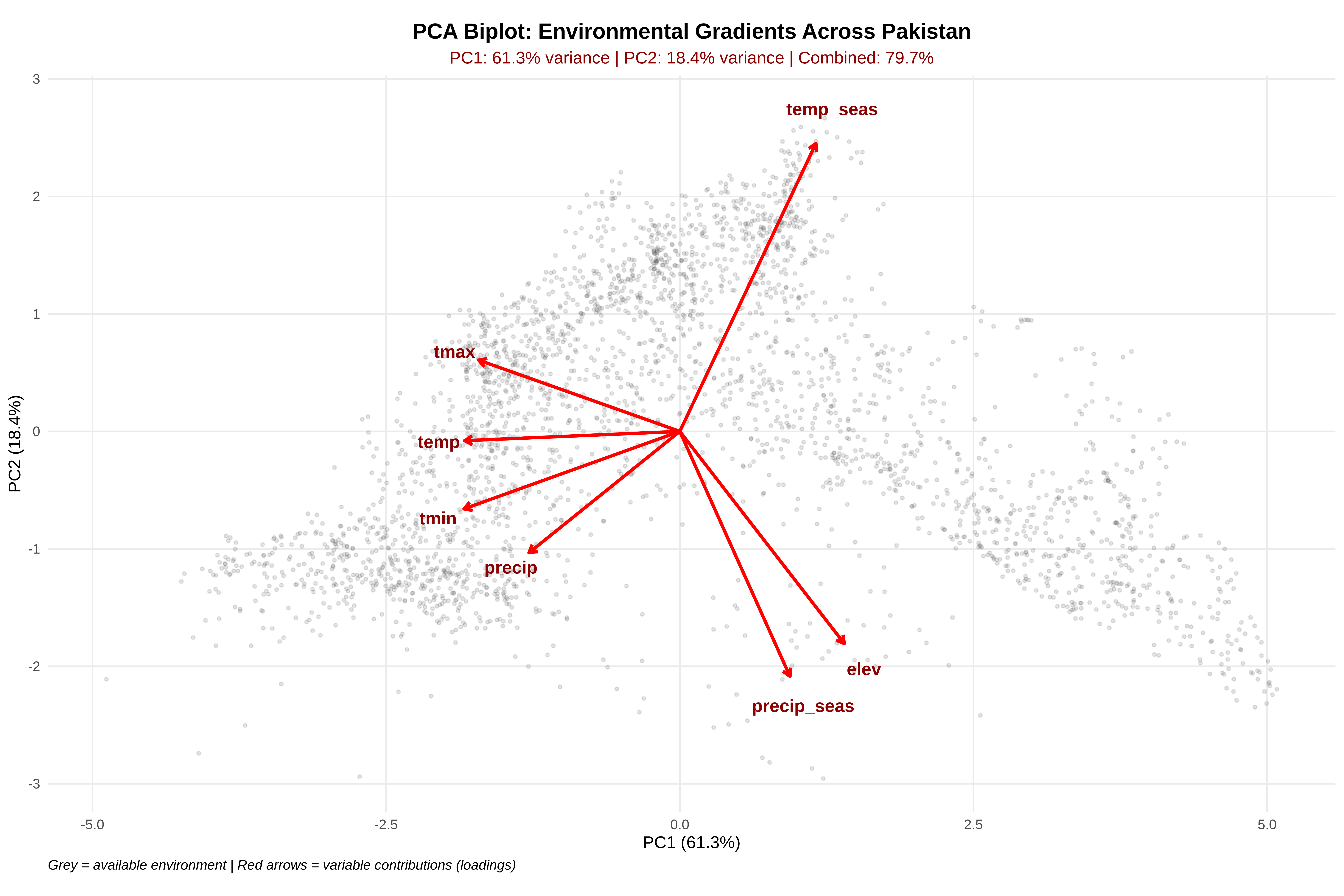
# --- Create PCA Biplot ---
# Extract scores (point positions in PC space) and loadings (variable arrows)
scores <- as.data.frame(pca$x[, 1:2])
load <- as.data.frame(pca$rotation[, 1:2])
load$var <- rownames(load)

# Determine scaling factor for arrows (so they're visible relative to points)
scale_factor <- min(
  (max(scores$PC1) - min(scores$PC1)) / (max(load$PC1) - min(load$PC1)),
  (max(scores$PC2) - min(scores$PC2)) / (max(load$PC2) - min(load$PC2))
) * 0.8

# Build biplot
p_biplot <- ggplot() +
  # Background points (available environment)
  geom_point(data = scores, aes(x = PC1, y = PC2),
             alpha = 0.15, size = 0.8, color = "gray30") +

  # Origin marker
  geom_point(x = 0, y = 0, size = 2, color = "red") +

  # Variable loading arrows
  geom_segment(data = load,
               aes(x = 0, y = 0,
                   xend = PC1 * scale_factor,
                   yend = PC2 * scale_factor),
               arrow = arrow(length = unit(0.2, "cm")),
               color = "red", linewidth = 1) +

  # Variable labels
  geom_text(data = load,
            aes(x = PC1 * scale_factor * 1.12,
                y = PC2 * scale_factor * 1.12,
                label = var),
            color = "darkred", size = 4, fontface = "bold") +

  # Axis labels with variance explained
  labs(
    title = "PCA Biplot: Environmental Gradients Across Pakistan",
    subtitle = paste0("PC1: ", var_exp[1], "% variance | PC2: ",
                     var_exp[2], "% variance | Combined: ",
                     cum_var[2], "%"),
    x = paste0("PC1 (", var_exp[1], "%)"),
    y = paste0("PC2 (", var_exp[2], "%)"),
    caption = "Grey = available environment | Red arrows = variable contributions (loadings)"
  ) +

  # Equal aspect ratio is essential for interpreting angles between arrows
  coord_fixed() +

  theme_minimal() +
  theme(
    plot.title = element_text(hjust = 0.5, face = "bold", size = 14),
    plot.subtitle = element_text(hjust = 0.5, color = "darkred", size = 11),
    plot.caption = element_text(hjust = 0, face = "italic"),
    panel.grid.minor = element_blank()
  )

print(p_biplot)

Code
# Save
ggsave(file.path(output_path, "s4_pca_biplot.png"),
       p_biplot, width = 10, height = 8, dpi = 300)
cat("✓ PCA biplot saved\n")

 ============================================================ 
PCA VARIANCE EXPLAINED
============================================================ 

Individual variance explained:
  PC1:  61.3% (cumulative:  61.3%)
  PC2:  18.4% (cumulative:  79.7%)
  PC3:  11.3% (cumulative:  91.0%)
  PC4:   5.3% (cumulative:  96.3%)
  PC5:   3.7% (cumulative:  99.9%)
  PC6:   0.1% (cumulative: 100.0%)
  PC7:   0.0% (cumulative: 100.0%)

First 2 PCs explain: 79.7% of total variance
First 3 PCs explain: 91.0% of total variance
✓ PCA biplot saved
What to Look For What It Means Ecological Implication
Arrows pointing same direction Positively correlated variables Measuring the same gradient (e.g., temp + tmax)
Arrows pointing opposite directions Negatively correlated Inverse relationship (e.g., temp vs elevation)
Arrows at 90° Uncorrelated variables Independent ecological information
Long arrows High loading on that PC Variable strongly contributes to that axis
Short arrows Low loading Variable poorly represented by first 2 PCs

Key Insight: PCA converts our 7 correlated climate variables (which caused VIF > 10 in Session 3) into uncorrelated axes. The biplot arrows show which original variables “define” each axis — temperature-related arrows are generally cluster together, confirming the collinearity we diagnosed earlier.

3. Loadings — “What Does Each PC Mean Biologically?”

Key Points:

  • High absolute loading = strong contribution to that PC

  • The sign indicates direction along the gradient (e.g., positive = warmer end)

  • Don’t over-interpret PCs with small variance explained (< 10%)

Code
# ==============================================================================
# STEP 7: INTERPRET PCA LOADINGS
# ==============================================================================
# Loadings tell us the "recipe" for each PC:
#   PC1 = 0.45 × temp + 0.42 × tmax + ... (a weighted combination)
# Variables with large absolute loadings define that axis

# Extract loadings for first 3 PCs
L <- as.data.frame(pca$rotation[, 1:3])
L$var <- rownames(L)

# Rename columns to include variance explained
colnames(L)[1:3] <- paste0("PC", 1:3, " (", var_exp[1:3], "%)")

# Reshape to long format for plotting
Llong <- tidyr::pivot_longer(L, -var, names_to = "PC", values_to = "loading")

# Create loading barplot
p_loadings <- ggplot(Llong, aes(x = reorder(var, loading), y = loading, fill = loading)) +
  geom_col(width = 0.7) +
  facet_wrap(~PC, ncol = 3) +
  scale_fill_gradient2(
    low = "darkred", mid = "white", high = "darkblue",
    midpoint = 0, name = "Loading"
  ) +
  coord_flip() +
  labs(
    title = "PCA Loadings: Interpreting Ecological Gradients",
    subtitle = "High absolute values indicate strong contribution to that PC axis",
    x = NULL,
    y = "Loading value"
  ) +
  theme_minimal() +
  theme(
    plot.title = element_text(hjust = 0.5, face = "bold", size = 14),
    plot.subtitle = element_text(hjust = 0.5, color = "darkred", size = 11),
    strip.text = element_text(face = "bold", size = 12),
    legend.position = "bottom",
    panel.grid.major.y = element_blank()
  )

print(p_loadings)

Code
# Save
ggsave(file.path(output_path, "s4_pca_loadings.png"),
       p_loadings, width = 10, height = 7, dpi = 300)
cat("✓ Loadings barplot saved\n")

# --- Print detailed interpretation ---
cat("\n", paste(rep("=", 70), collapse = ""), "\n")
cat("INTERPRETATION OF PCA LOADINGS\n")
cat(paste(rep("=", 70), collapse = ""), "\n\n")

loadings_mat <- pca$rotation[, 1:3]

for(pc_idx in 1:3) {
  pc_name <- paste0("PC", pc_idx)
  pc_var <- var_exp[pc_idx]

  # Sort by absolute loading
  sorted_vars <- names(sort(abs(loadings_mat[, pc_idx]), decreasing = TRUE))

  cat(sprintf("%s (%.1f%% of variance):\n", pc_name, pc_var))
  for(v in sorted_vars) {
    val <- loadings_mat[v, pc_idx]
    bar <- paste(rep(ifelse(val > 0, "+", "-"), round(abs(val) * 20)), collapse = "")
    cat(sprintf("  %-12s: %+.3f  %s\n", v, val, bar))
  }

  # Suggest ecological interpretation
  top_vars <- sorted_vars[1:3]
  if(any(grepl("temp|tmax|tmin", paste(top_vars, collapse = "|")))) {
    cat("  → Likely represents: ENERGY / TEMPERATURE gradient\n\n")
  } else if(any(grepl("precip|prec", paste(top_vars, collapse = "|")))) {
    cat("  → Likely represents: MOISTURE / PRECIPITATION gradient\n\n")
  } else if(any(grepl("elev", paste(top_vars, collapse = "|")))) {
    cat("  → Likely represents: TOPOGRAPHIC / ELEVATIONAL gradient\n\n")
  } else {
    cat("  → Interpretation requires domain knowledge\n\n")
  }
}
✓ Loadings barplot saved

 ====================================================================== 
INTERPRETATION OF PCA LOADINGS
====================================================================== 

PC1 (61.3% of variance):
  tmin        : -0.467  ---------
  temp        : -0.465  ---------
  tmax        : -0.435  ---------
  elev        : +0.356  +++++++
  precip      : -0.326  -------
  temp_seas   : +0.294  ++++++
  precip_seas : +0.238  +++++
  → Likely represents: ENERGY / TEMPERATURE gradient

PC2 (18.4% of variance):
  temp_seas   : +0.623  ++++++++++++
  precip_seas : -0.530  -----------
  elev        : -0.459  ---------
  precip      : -0.263  -----
  tmin        : -0.168  ---
  tmax        : +0.154  +++
  temp        : -0.020  
  → Likely represents: ENERGY / TEMPERATURE gradient

PC3 (11.3% of variance):
  precip      : -0.608  ------------
  precip_seas : +0.602  ++++++++++++
  tmax        : +0.379  ++++++++
  temp        : +0.266  +++++
  temp_seas   : +0.154  +++
  tmin        : +0.151  +++
  elev        : -0.078  --
  → Likely represents: ENERGY / TEMPERATURE gradient

Interpretation Guide

Loading Value Meaning Example
+0.40 to +0.50 Strong positive contribution Variable increases along positive end of that PC
-0.40 to -0.50 Strong negative contribution Variable increases along negative end of that PC
-0.10 to +0.10 Weak contribution Variable is not well-represented by this PC

Key Insight: PC1 typically captures the strongest environmental gradient in the data. In Pakistan, this is usually a temperature–elevation gradient (hot lowlands ↔︎ cold mountains). PC2 often captures moisture variation. The loadings let you translate abstract “PC axes” into meaningful ecological language.

4. Climate Niche Space — Where Presences Sit in PCA Space

Key Points:

  • Compare available environment (what’s out there) vs used environment (where the species occurs)

  • Sampling bias can distort niche inference — presence in a region of PCA space could reflect sampling effort, not preference

  • Useful for diagnosing extrapolation risk: if presences cluster tightly, predictions outside that region are unreliable

Code
# ==============================================================================
# STEP 8: PROJECT PRESENCES INTO PCA SPACE
# ==============================================================================
# IMPORTANT: We scale presences using the SAME parameters as the background
# (same center, same standard deviation). This ensures they're in the same space.

# Scale presences using background scaling parameters
pres_scaled <- scale(pres_env,
                     center = scale_center,
                     scale = scale_sd)

# Project presences into PCA space using background rotation matrix
pres_scores <- as.data.frame(pres_scaled %*% pca$rotation[, 1:2])
names(pres_scores) <- c("PC1", "PC2")
pres_scores$type <- "Presence"

# Get background scores
avail_scores <- as.data.frame(pca$x[, 1:2])
avail_scores$type <- "Available"

# --- 2D kernel density for available environment ---
kde <- kde2d(avail_scores$PC1, avail_scores$PC2, n = 100)
kde_df <- expand.grid(PC1 = kde$x, PC2 = kde$y)
kde_df$density <- as.vector(kde$z)

# --- Create niche plot ---
p_niche <- ggplot() +
  # Density contours for available environment
  geom_contour(data = kde_df,
               aes(x = PC1, y = PC2, z = density, color = after_stat(level)),
               bins = 10, alpha = 0.6) +

  # Available environment points (grey)
  geom_point(data = avail_scores,
             aes(x = PC1, y = PC2),
             alpha = 0.1, size = 0.7, color = "gray30") +

  # Presence points (red)
  geom_point(data = pres_scores,
             aes(x = PC1, y = PC2),
             color = "red", alpha = 0.7, size = 2) +

  # Density polygons for presences
  stat_density2d(data = pres_scores,
                 aes(x = PC1, y = PC2, fill = after_stat(level)),
                 alpha = 0.3, geom = "polygon", bins = 5) +

  scale_fill_viridis_c(option = "plasma", name = "Presence\ndensity") +
  scale_color_viridis_c(option = "viridis", name = "Available\ndensity") +

  labs(
    title = "Climate Niche Space — Spider Presences vs Available Environment",
    subtitle = paste0("Red = Presences (n=", nrow(pres_scores), ") | ",
                     "Grey = Available (n=", nrow(avail_scores), ") | ",
                     "Contours show density"),
    x = paste0("PC1 (", var_exp[1], "%)"),
    y = paste0("PC2 (", var_exp[2], "%)"),
    caption = "Presences occupying a subset of available space suggests niche specialization or sampling bias"
  ) +

  coord_fixed() +
  theme_minimal() +
  theme(
    plot.title = element_text(hjust = 0.5, face = "bold", size = 14),
    plot.subtitle = element_text(hjust = 0.5, size = 10),
    plot.caption = element_text(hjust = 0, face = "italic"),
    legend.position = "right"
  )

print(p_niche)

Code
# Save
ggsave(file.path(output_path, "s4_niche_pca.png"),
       p_niche, width = 10, height = 8, dpi = 300)
cat("✓ Climate niche space plot saved\n")
✓ Climate niche space plot saved
Code
# ==============================================================================
# STEP 9: CALCULATE NICHE METRICS
# ==============================================================================
# Quantify how the species' niche relates to available climate space

cat("\n", paste(rep("=", 60), collapse = ""), "\n")
cat("NICHE METRICS IN PCA SPACE\n")
cat(paste(rep("=", 60), collapse = ""), "\n\n")

# --- 9a: Proportion of presences within available range ---
range_PC1 <- range(avail_scores$PC1)
range_PC2 <- range(avail_scores$PC2)

pres_in_range <- sum(
  pres_scores$PC1 >= range_PC1[1] & pres_scores$PC1 <= range_PC1[2] &
  pres_scores$PC2 >= range_PC2[1] & pres_scores$PC2 <= range_PC2[2]
)

cat("1. CONTAINMENT:\n")
cat(sprintf("   Presences within available climate range: %d/%d (%.1f%%)\n",
            pres_in_range, nrow(pres_scores),
            100 * pres_in_range / nrow(pres_scores)))
cat("   → Values < 100% indicate potential extrapolation risk\n\n")

# --- 9b: Centroid shift ---
centroid_avail <- colMeans(avail_scores[, 1:2])
centroid_pres <- colMeans(pres_scores[, 1:2])
shift_dist <- sqrt(sum((centroid_pres - centroid_avail)^2))

cat("2. CENTROID SHIFT (available → presence):\n")
cat(sprintf("   Available centroid: PC1 = %.2f, PC2 = %.2f\n",
            centroid_avail[1], centroid_avail[2]))
cat(sprintf("   Presence centroid:  PC1 = %.2f, PC2 = %.2f\n",
            centroid_pres[1], centroid_pres[2]))
cat(sprintf("   Euclidean shift: %.2f PC units\n", shift_dist))
cat("   → Large shift = species occupies non-average climate\n\n")

# --- 9c: Niche breadth (spread in PC space) ---
avail_spread <- apply(avail_scores[, 1:2], 2, sd)
pres_spread <- apply(pres_scores[, 1:2], 2, sd)

cat("3. NICHE BREADTH (standard deviation in PC space):\n")
cat(sprintf("   Available SD:  PC1 = %.2f, PC2 = %.2f\n",
            avail_spread[1], avail_spread[2]))
cat(sprintf("   Presence SD:   PC1 = %.2f, PC2 = %.2f\n",
            pres_spread[1], pres_spread[2]))
cat(sprintf("   Breadth ratio: PC1 = %.1f%%, PC2 = %.1f%%\n",
            100 * pres_spread[1] / avail_spread[1],
            100 * pres_spread[2] / avail_spread[2]))
cat("   → Ratio < 50% suggests narrow niche or biased sampling\n")

 ============================================================ 
NICHE METRICS IN PCA SPACE
============================================================ 

1. CONTAINMENT:
   Presences within available climate range: 93/93 (100.0%)
   → Values < 100% indicate potential extrapolation risk

2. CENTROID SHIFT (available → presence):
   Available centroid: PC1 = 0.00, PC2 = 0.00
   Presence centroid:  PC1 = -1.49, PC2 = -0.10
   Euclidean shift: 1.50 PC units
   → Large shift = species occupies non-average climate

3. NICHE BREADTH (standard deviation in PC space):
   Available SD:  PC1 = 2.07, PC2 = 1.13
   Presence SD:   PC1 = 0.05, PC2 = 0.12
   Breadth ratio: PC1 = 2.3%, PC2 = 10.4%
   → Ratio < 50% suggests narrow niche or biased sampling

Interpretation Guide

Niche Metric What It Tells You What to Watch For
Containment (< 100%) Presences outside available range Extrapolation risk: model predicts beyond training data
Centroid shift (large) Species occupies non-average climate Could indicate true preference OR sampling bias
Breadth ratio (< 50%) Species uses narrow subset of available climate Specialization, or sampling restricted to certain areas

Key Insight: If presences cluster tightly in one corner of PCA space, it could mean the species is a specialist — or that sampling was concentrated in certain climate zones (e.g., near roads in lowlands). Session 3’s sampling bias analysis helps distinguish these explanations.

5. UMAP — Nonlinear Visualization of Environmental Space

Key Points:

  • UMAP (Uniform Manifold Approximation and Projection) captures nonlinear relationships that PCA misses

  • Great for revealing clusters, gradients, and non-obvious structure

  • NOT for inference: axes have no inherent meaning, results depend on tuning parameters

  • Use as a complement to PCA, not a replacement

Code
# ==============================================================================
# STEP 10: UMAP VISUALIZATION
# ==============================================================================
# We run UMAP on the same scaled background data used for PCA
# Two parameter sets show how tuning affects the visualization

cat("Running UMAP embeddings (this may take a few seconds)...\n")

# --- 10a: UMAP with local structure emphasis ---
set.seed(42)
emb_local <- umap(avail_scaled,
                   n_neighbors = 15,   # Fewer neighbors = focus on local structure
                   min_dist = 0.1,     # Small = tighter clusters
                   metric = "euclidean")

# --- 10b: UMAP with global structure emphasis ---
set.seed(42)
emb_global <- umap(avail_scaled,
                    n_neighbors = 50,   # More neighbors = focus on global structure
                    min_dist = 0.5,     # Larger = more spread out
                    metric = "euclidean")

cat("✓ Both UMAP embeddings computed\n")

# --- Create data frames for plotting ---
df_local <- data.frame(
  UMAP1 = emb_local[, 1],
  UMAP2 = emb_local[, 2],
  temp = avail_env$temp,
  precip = avail_env$precip,
  elev = avail_env$elev
)

df_global <- data.frame(
  UMAP1 = emb_global[, 1],
  UMAP2 = emb_global[, 2],
  temp = avail_env$temp,
  precip = avail_env$precip,
  elev = avail_env$elev
)

# --- Plot 1: Local structure, colored by temperature ---
p_umap_local <- ggplot(df_local, aes(x = UMAP1, y = UMAP2, color = temp)) +
  geom_point(alpha = 0.5, size = 1.2) +
  scale_color_viridis_c(option = "plasma", name = "Temp (°C)") +
  labs(
    title = "UMAP — Local Structure",
    subtitle = "n_neighbors = 15, min_dist = 0.1",
    x = "UMAP1", y = "UMAP2"
  ) +
  theme_minimal() +
  theme(
    plot.title = element_text(hjust = 0.5, face = "bold", size = 12),
    plot.subtitle = element_text(hjust = 0.5, size = 10),
    legend.position = "right"
  )

# --- Plot 2: Global structure, colored by temperature ---
p_umap_global <- ggplot(df_global, aes(x = UMAP1, y = UMAP2, color = temp)) +
  geom_point(alpha = 0.5, size = 1.2) +
  scale_color_viridis_c(option = "plasma", name = "Temp (°C)") +
  labs(
    title = "UMAP — Global Structure",
    subtitle = "n_neighbors = 50, min_dist = 0.5",
    x = "UMAP1", y = "UMAP2"
  ) +
  theme_minimal() +
  theme(
    plot.title = element_text(hjust = 0.5, face = "bold", size = 12),
    plot.subtitle = element_text(hjust = 0.5, size = 10),
    legend.position = "right"
  )

# --- Combine ---
p_umap_combined <- p_umap_local + p_umap_global +
  plot_annotation(
    title = "UMAP: Nonlinear Visualization of Pakistan's Environmental Space",
    subtitle = "Parameter tuning affects whether local clusters or global gradients are emphasized",
    theme = theme(
      plot.title = element_text(hjust = 0.5, face = "bold", size = 14),
      plot.subtitle = element_text(hjust = 0.5, size = 11)
    )
  )

print(p_umap_combined)

Code
# Save
ggsave(file.path(output_path, "s4_umap_comparison.png"),
       p_umap_combined, width = 14, height = 6, dpi = 300)
cat("✓ UMAP comparison plot saved\n")
Running UMAP embeddings (this may take a few seconds)...
✓ Both UMAP embeddings computed
✓ UMAP comparison plot saved

Interpretation Guide

UMAP Feature What It Means Caution
Distinct clusters Groups of similar environments Could be artifact of parameter choice
Smooth color gradient UMAP preserves that environmental gradient Good — validates ecological structure
Fragmented colors That variable is not well-captured by UMAP May need different parameters or more dimensions
Different results with different parameters UMAP is sensitive to tuning Always try multiple settings; never rely on a single run

Key Insight: UMAP is a powerful visualization tool, but it is not a statistical model. The axes (UMAP1, UMAP2) have no units and no inherent meaning. Use UMAP to explore and discover patterns, then use PCA or formal models to test them.


6. PCA vs UMAP — When to Use Each

Code
# ==============================================================================
# STEP 12: PRINT COMPARISON TABLE
# ==============================================================================

cat("\n", paste(rep("=", 80), collapse = ""), "\n")
cat("PCA vs UMAP: WHEN TO USE EACH\n")
cat(paste(rep("=", 80), collapse = ""), "\n\n")

comparison <- data.frame(
  Feature = c("Type", "Axes meaning", "Reproducible?",
              "Handles nonlinear?", "Good for inference?",
              "Good for visualization?", "Tuning needed?",
              "Best for SDMs?"),
  PCA = c("Linear", "Interpretable (loadings)", "Yes (deterministic)",
          "No", "Yes (with caution)", "Yes (first 2-3 PCs)",
          "No (just choose # of PCs)", "Yes — uncorrelated predictors"),
  UMAP = c("Nonlinear", "No inherent meaning", "No (depends on seed + params)",
           "Yes", "No", "Yes (excellent)",
           "Yes (n_neighbors, min_dist)", "No — use for exploration only"),
  check.names = FALSE
)

print(comparison, row.names = FALSE)

cat("\n", paste(rep("-", 80), collapse = ""), "\n")
cat("PRACTICAL RECOMMENDATIONS:\n")
cat(paste(rep("-", 80), collapse = ""), "\n")
cat("• For SDM predictor preparation → PCA (creates uncorrelated axes)\n")
cat("• For niche analysis → PCA (interpretable, comparable across studies)\n")
cat("• For exploring high-dimensional structure → UMAP (reveals clusters)\n")
cat("• For publication figures → Both (PCA for rigor, UMAP for visual appeal)\n")
cat("• NEVER use UMAP axes as model predictors\n")

 ================================================================================ 
PCA vs UMAP: WHEN TO USE EACH
================================================================================ 

                 Feature                           PCA
                    Type                        Linear
            Axes meaning      Interpretable (loadings)
           Reproducible?           Yes (deterministic)
      Handles nonlinear?                            No
     Good for inference?            Yes (with caution)
 Good for visualization?           Yes (first 2-3 PCs)
          Tuning needed?     No (just choose # of PCs)
          Best for SDMs? Yes — uncorrelated predictors
                          UMAP
                     Nonlinear
           No inherent meaning
 No (depends on seed + params)
                           Yes
                            No
               Yes (excellent)
   Yes (n_neighbors, min_dist)
 No — use for exploration only

 -------------------------------------------------------------------------------- 
PRACTICAL RECOMMENDATIONS:
-------------------------------------------------------------------------------- 
• For SDM predictor preparation → PCA (creates uncorrelated axes)
• For niche analysis → PCA (interpretable, comparable across studies)
• For exploring high-dimensional structure → UMAP (reveals clusters)
• For publication figures → Both (PCA for rigor, UMAP for visual appeal)
• NEVER use UMAP axes as model predictors

7. Complete Practical Workflow

Code
# ==============================================================================
# STEP 13: COMPLETE SESSION 4 WORKFLOW SUMMARY
# ==============================================================================

cat("\n", paste(rep("=", 70), collapse = ""), "\n")
cat("SESSION 4: MULTIVARIATE & DIMENSIONALITY REDUCTION — COMPLETE WORKFLOW\n")
cat(paste(rep("=", 70), collapse = ""), "\n")

# 1) PCA Summary
cat("\n1. PCA SUMMARY\n")
cat(paste(rep("-", 40), collapse = ""), "\n")
cat(sprintf("   Variables used: %s\n", paste(short_names, collapse = ", ")))
cat(sprintf("   PC1 explains: %.1f%% of variance\n", var_exp[1]))
cat(sprintf("   PC2 explains: %.1f%% of variance\n", var_exp[2]))
cat(sprintf("   First 2 PCs combined: %.1f%%\n", cum_var[2]))
cat(sprintf("   First 3 PCs combined: %.1f%%\n\n", cum_var[3]))

# 2) Loadings Summary
cat("2. DOMINANT LOADINGS\n")
cat(paste(rep("-", 40), collapse = ""), "\n")
for(pc_idx in 1:2) {
  top_var <- names(which.max(abs(pca$rotation[, pc_idx])))
  top_val <- pca$rotation[top_var, pc_idx]
  cat(sprintf("   PC%d top loading: %s (%.3f)\n", pc_idx, top_var, top_val))
}

# 3) Niche Position
cat("\n3. NICHE POSITION\n")
cat(paste(rep("-", 40), collapse = ""), "\n")
cat(sprintf("   Centroid shift: %.2f PC units\n", shift_dist))
cat(sprintf("   Niche breadth (PC1): %.1f%% of available\n",
            100 * pres_spread[1] / avail_spread[1]))
cat(sprintf("   Niche breadth (PC2): %.1f%% of available\n",
            100 * pres_spread[2] / avail_spread[2]))

# 4) Files saved
cat("\n4. OUTPUT FILES\n")
cat(paste(rep("-", 40), collapse = ""), "\n")
cat("   ", file.path(output_path, "s4_pca_biplot.png"), "\n")
cat("   ", file.path(output_path, "s4_pca_loadings.png"), "\n")
cat("   ", file.path(output_path, "s4_niche_pca.png"), "\n")
cat("   ", file.path(output_path, "s4_umap_comparison.png"), "\n")
cat("   ", file.path(output_path, "s4_umap_multi_variable.png"), "\n")

cat("\n", paste(rep("=", 70), collapse = ""), "\n")
cat("Session 4 complete!\n")
cat(paste(rep("=", 70), collapse = ""), "\n")

 ====================================================================== 
SESSION 4: MULTIVARIATE & DIMENSIONALITY REDUCTION — COMPLETE WORKFLOW
====================================================================== 

1. PCA SUMMARY
---------------------------------------- 
   Variables used: temp, tmax, tmin, temp_seas, precip, precip_seas, elev
   PC1 explains: 61.3% of variance
   PC2 explains: 18.4% of variance
   First 2 PCs combined: 79.7%
   First 3 PCs combined: 91.0%

2. DOMINANT LOADINGS
---------------------------------------- 
   PC1 top loading: tmin (-0.467)
   PC2 top loading: temp_seas (0.623)

3. NICHE POSITION
---------------------------------------- 
   Centroid shift: 1.50 PC units
   Niche breadth (PC1): 2.3% of available
   Niche breadth (PC2): 10.4% of available

4. OUTPUT FILES
---------------------------------------- 
    /run/media/tahirali/Expansion/github/spatial-ecology-workshop/output/Session_4/s4_pca_biplot.png 
    /run/media/tahirali/Expansion/github/spatial-ecology-workshop/output/Session_4/s4_pca_loadings.png 
    /run/media/tahirali/Expansion/github/spatial-ecology-workshop/output/Session_4/s4_niche_pca.png 
    /run/media/tahirali/Expansion/github/spatial-ecology-workshop/output/Session_4/s4_umap_comparison.png 
    /run/media/tahirali/Expansion/github/spatial-ecology-workshop/output/Session_4/s4_umap_multi_variable.png 

 ====================================================================== 
Session 4 complete!
====================================================================== 

8. Reasoning Prompts

Code
# ==============================================================================
# STEP 14: ECOLOGICAL REASONING PROMPTS
# ==============================================================================

cat("\n", paste(rep("=", 70), collapse = ""), "\n")
cat("REASONING PROMPTS FOR DISCUSSION\n")
cat(paste(rep("=", 70), collapse = ""), "\n\n")

cat("1. If PC1 is mostly temperature variables, what ecological gradient is that?\n")
cat("   → Energy/temperature gradient (affects metabolic rates, growing season,\n")
cat("     physiological limits). In Pakistan, this tracks the Himalayan\n")
cat("     elevation gradient: hot plains → cold mountains.\n\n")

cat("2. If presences occupy only a small region of available PCA space,\n")
cat("   does that mean specialization, sampling bias, or dispersal limitation?\n")
cat("   • Specialization: Narrow fundamental niche (species can only tolerate\n")
cat("     specific conditions)\n")
cat("   • Sampling bias: Only surveyed accessible areas (roads, lowlands)\n")
cat("   • Dispersal limitation: Species hasn't reached all suitable areas\n")
cat("   → Need independent data to distinguish (e.g., experimental tolerances,\n")
cat("     surveys in remote areas, SDMs with bias correction)\n\n")

cat("3. Why should we NOT use UMAP axes as predictors in an SDM?\n")
cat("   • UMAP axes have no consistent meaning across runs\n")
cat("   • The mapping is non-invertible (can't project new data reliably)\n")
cat("   • Results depend on arbitrary parameter choices\n")
cat("   → Use PCA for creating model inputs; use UMAP for exploration only\n\n")

cat("4. How does PCA relate to the VIF analysis from Session 3?\n")
cat("   • VIF measured how correlated each variable was with ALL others\n")
cat("   • PCA solves the same problem by creating NEW uncorrelated variables\n")
cat("   • PC scores can be used as predictors in SDMs without collinearity\n")
cat("   • Trade-off: PCA axes are harder to interpret ecologically\n\n")

cat("5. When would you choose PCA + SDM over Elastic Net + original variables?\n")
cat("   • When you have MANY (>15) correlated predictors\n")
cat("   • When ecological interpretation of individual variables is less important\n")
cat("   • When you want to visualize the niche in reduced space\n")
cat("   • Elastic Net is better when you want to know WHICH variables matter\n")

 ====================================================================== 
REASONING PROMPTS FOR DISCUSSION
====================================================================== 

1. If PC1 is mostly temperature variables, what ecological gradient is that?
   → Energy/temperature gradient (affects metabolic rates, growing season,
     physiological limits). In Pakistan, this tracks the Himalayan
     elevation gradient: hot plains → cold mountains.

2. If presences occupy only a small region of available PCA space,
   does that mean specialization, sampling bias, or dispersal limitation?
   • Specialization: Narrow fundamental niche (species can only tolerate
     specific conditions)
   • Sampling bias: Only surveyed accessible areas (roads, lowlands)
   • Dispersal limitation: Species hasn't reached all suitable areas
   → Need independent data to distinguish (e.g., experimental tolerances,
     surveys in remote areas, SDMs with bias correction)

3. Why should we NOT use UMAP axes as predictors in an SDM?
   • UMAP axes have no consistent meaning across runs
   • The mapping is non-invertible (can't project new data reliably)
   • Results depend on arbitrary parameter choices
   → Use PCA for creating model inputs; use UMAP for exploration only

4. How does PCA relate to the VIF analysis from Session 3?
   • VIF measured how correlated each variable was with ALL others
   • PCA solves the same problem by creating NEW uncorrelated variables
   • PC scores can be used as predictors in SDMs without collinearity
   • Trade-off: PCA axes are harder to interpret ecologically

5. When would you choose PCA + SDM over Elastic Net + original variables?
   • When you have MANY (>15) correlated predictors
   • When ecological interpretation of individual variables is less important
   • When you want to visualize the niche in reduced space
   • Elastic Net is better when you want to know WHICH variables matter

9. Session Summary

Code
# ==============================================================================
# SESSION 4 SUMMARY
# ==============================================================================

cat("\n", paste(rep("=", 70), collapse = ""), "\n")
cat("SESSION 4 SUMMARY: KEY TAKEAWAYS\n")
cat(paste(rep("=", 70), collapse = ""), "\n\n")

cat("1. PCA AS GRADIENT ANALYSIS:\n")
cat("   • PCA converts correlated climate variables into uncorrelated axes\n")
cat("   • Each axis represents an ecological gradient (energy, moisture, etc.)\n")
cat("   • First 2-3 PCs typically capture >80% of environmental variation\n\n")

cat("2. LOADINGS = ECOLOGICAL MEANING:\n")
cat("   • Loadings tell you which variables define each PC\n")
cat("   • Temperature variables cluster → temperature gradient\n")
cat("   • Precipitation variables cluster → moisture gradient\n")
cat("   • Essential for translating statistical axes into biology\n\n")

cat("3. CLIMATE NICHE SPACE:\n")
cat("   • Presences vs available environment reveals niche position\n")
cat("   • Centroid shift = non-random habitat use\n")
cat("   • Narrow niche breadth = specialization OR sampling bias\n")
cat("   • Always consider bias before interpreting as preference\n\n")

cat("4. UMAP FOR EXPLORATION:\n")
cat("   • Captures nonlinear structure PCA misses\n")
cat("   • Excellent for visualization and pattern discovery\n")
cat("   • Parameter-dependent and non-reproducible → not for inference\n")
cat("   • Use alongside PCA, never as a replacement\n\n")

cat("5. CONNECTION TO PREVIOUS SESSIONS:\n")
cat("   • Session 3 VIF > 10 → PCA creates uncorrelated alternatives\n")
cat("   • Session 3 Elastic Net selects variables → PCA combines them\n")
cat("   • Both approaches handle collinearity; choice depends on goals\n")

cat("\n", paste(rep("=", 70), collapse = ""), "\n")

 ====================================================================== 
SESSION 4 SUMMARY: KEY TAKEAWAYS
====================================================================== 

1. PCA AS GRADIENT ANALYSIS:
   • PCA converts correlated climate variables into uncorrelated axes
   • Each axis represents an ecological gradient (energy, moisture, etc.)
   • First 2-3 PCs typically capture >80% of environmental variation

2. LOADINGS = ECOLOGICAL MEANING:
   • Loadings tell you which variables define each PC
   • Temperature variables cluster → temperature gradient
   • Precipitation variables cluster → moisture gradient
   • Essential for translating statistical axes into biology

3. CLIMATE NICHE SPACE:
   • Presences vs available environment reveals niche position
   • Centroid shift = non-random habitat use
   • Narrow niche breadth = specialization OR sampling bias
   • Always consider bias before interpreting as preference

4. UMAP FOR EXPLORATION:
   • Captures nonlinear structure PCA misses
   • Excellent for visualization and pattern discovery
   • Parameter-dependent and non-reproducible → not for inference
   • Use alongside PCA, never as a replacement

5. CONNECTION TO PREVIOUS SESSIONS:
   • Session 3 VIF > 10 → PCA creates uncorrelated alternatives
   • Session 3 Elastic Net selects variables → PCA combines them
   • Both approaches handle collinearity; choice depends on goals

 ====================================================================== 

Bridge to Session 5: Species Distribution Modeling

What We Learned in Session 4:

  • PCA axes are uncorrelated summaries of environmental gradients

  • Loadings let us interpret what each axis means ecologically

  • Climate niche space shows where presences sit relative to available conditions

  • UMAP reveals nonlinear structure but is not suitable for modeling

How This Connects to Session 5:

1. PCA scores as SDM predictors

  • Use PC1, PC2, (PC3) as uncorrelated inputs to SDMs

  • Eliminates the collinearity problem diagnosed in Session 3

  • Trade-off: harder to interpret response curves

2. Niche space informs model evaluation

  • If presences cluster in PCA space → model should predict high suitability there

  • If available environment extends far beyond presences → check for extrapolation

  • Niche breadth metrics help set expectations for model performance

3. Comparing approaches

  • Session 3 approach: Elastic Net with original variables (interpretable but collinear)

  • Session 4 approach: PCA scores as predictors (uncorrelated but abstract)

  • Session 5 will use both and compare model performance

Session Info for Reproducibility

Code
# For reproducibility
cat("\n=== SESSION INFO ===\n")
print(sessionInfo())

=== SESSION INFO ===
R version 4.4.3 (2025-02-28)
Platform: x86_64-conda-linux-gnu
Running under: Fedora Linux 39 (Workstation Edition)

Matrix products: default
BLAS/LAPACK: /run/media/tahirali/2a4efc98-aaa3-4a01-a063-37db1463f3a8/tools/anaconda/envs/quarto-env/lib/libopenblasp-r0.3.30.so;  LAPACK version 3.12.0

locale:
 [1] LC_CTYPE=en_US.UTF-8       LC_NUMERIC=C              
 [3] LC_TIME=en_US.UTF-8        LC_COLLATE=en_US.UTF-8    
 [5] LC_MONETARY=en_US.UTF-8    LC_MESSAGES=en_US.UTF-8   
 [7] LC_PAPER=en_US.UTF-8       LC_NAME=C                 
 [9] LC_ADDRESS=C               LC_TELEPHONE=C            
[11] LC_MEASUREMENT=en_US.UTF-8 LC_IDENTIFICATION=C       

time zone: Europe/Berlin
tzcode source: system (glibc)

attached base packages:
[1] stats     graphics  grDevices utils     datasets  methods   base     

other attached packages:
 [1] uwot_0.2.4        Matrix_1.7-4      MASS_7.3-65       patchwork_1.3.2  
 [5] viridis_0.6.5     viridisLite_0.4.2 sf_1.1-0          terra_1.8-70     
 [9] tidyr_1.3.1       dplyr_1.1.4       ggplot2_4.0.0    

loaded via a namespace (and not attached):
 [1] generics_0.1.4     class_7.3-23       KernSmooth_2.23-26 lattice_0.22-7    
 [5] digest_0.6.37      magrittr_2.0.4     evaluate_1.0.5     grid_4.4.3        
 [9] RColorBrewer_1.1-3 fastmap_1.2.0      jsonlite_2.0.0     RSpectra_0.16-2   
[13] e1071_1.7-16       DBI_1.2.3          gridExtra_2.3      purrr_1.1.0       
[17] scales_1.4.0       isoband_0.2.7      textshaping_1.0.3  codetools_0.2-20  
[21] cli_3.6.5          rlang_1.1.6        units_0.8-7        withr_3.0.2       
[25] yaml_2.3.10        FNN_1.1.4.1        tools_4.4.3        vctrs_0.6.5       
[29] R6_2.6.1           proxy_0.4-27       lifecycle_1.0.4    classInt_0.4-11   
[33] htmlwidgets_1.6.4  ragg_1.5.0         pkgconfig_2.0.3    pillar_1.11.1     
[37] gtable_0.3.6       glue_1.8.0         Rcpp_1.1.0         systemfonts_1.3.1 
[41] xfun_0.53          tibble_3.3.0       tidyselect_1.2.1   knitr_1.50        
[45] farver_2.1.2       htmltools_0.5.8.1  rmarkdown_2.30     labeling_0.4.3    
[49] compiler_4.4.3     S7_0.2.0