Session 5: Species Distribution Modeling — GLM/GAM + ML + Spatial CV

Advanced Spatial Ecology & Species Distribution Modeling

Author

Dr Tahir Ali | AG de Meaux | TRR341 Ecological Genomics | University of Cologne

Code
# Setup chunk - runs before everything else
knitr::opts_chunk$set(echo = TRUE, message = FALSE, warning = FALSE)

# Create output directory if it doesn't exist
output_dir <- "/run/media/tahirali/Expansion/github/spatial-ecology-workshop/output/Session_5"
dir.create(output_dir, showWarnings = FALSE, recursive = TRUE)

Session Overview

Learning Outcomes:

  • Fit SDMs using GLM, GAM, Random Forest, and MaxEnt-like (maxnet)

  • Use spatial cross-validation to avoid over-optimistic accuracy

  • Interpret variable importance and biological plausibility

  • Produce prediction maps with uncertainty-aware thinking

🔗 Connection to Sessions 3 & 4:

  • Session 3 taught us to diagnose collinearity (VIF) and use regularization (Elastic Net) to select variables → we apply those methods here to choose SDM predictors

  • Session 4 showed us how PCA creates uncorrelated environmental axes → we compare SDMs built with original variables vs PCA scores

  • This session brings everything together: selected variables + appropriate models + honest evaluation

Code
# ==============================================================================
# STEP 1: LOAD REQUIRED PACKAGES
# ==============================================================================
# All packages from Sessions 3 & 4 plus SDM-specific tools

library(ggplot2)      # Professional plots
library(dplyr)        # Data manipulation
library(tidyr)        # Reshaping data
library(terra)        # Raster data
library(sf)           # Spatial vector data
library(viridis)      # Color-blind friendly palettes
library(patchwork)    # Combining plots

# Session 3 tools (variable selection)
library(car)          # VIF calculation
library(glmnet)       # Regularization (LASSO, Ridge, Elastic Net)

# Session 5 tools (SDMs)
library(mgcv)         # GAMs with smooth terms
library(ranger)       # Fast Random Forest implementation
library(maxnet)       # MaxEnt-like modeling in R
library(pROC)         # AUC calculation
library(MASS)         # Multivariate statistics (kde2d)

# Set seed for reproducibility
set.seed(123)

PART 1: LOAD AND PREPARE DATA (Limited to Pakistan)

(Same Pipeline as Sessions 3 & 4)

Code
# ==============================================================================
# STEP 2: DEFINE FILE PATHS
# ==============================================================================
# Same paths as Sessions 3 & 4

base_path <- "/run/media/tahirali/Expansion/github/spatial-ecology-workshop/"

spider_coords_path <- file.path(base_path, "data/presence/spider_coords.csv")
climate_folder <- file.path(base_path, "data/climate")
boundary_path <- file.path(base_path, "data/boundaries/pakistan_admin.shp")

output_path <- file.path(base_path, "output/Session_5")
dir.create(output_path, showWarnings = FALSE, recursive = TRUE)

cat("✓ File paths defined\n")
cat("  Input data: ", base_path, "\n")
cat("  Output directory: ", output_path, "\n")
✓ File paths defined
  Input data:  /run/media/tahirali/Expansion/github/spatial-ecology-workshop/ 
  Output directory:  /run/media/tahirali/Expansion/github/spatial-ecology-workshop//output/Session_5 
Code
# ==============================================================================
# STEP 3: LOAD SPIDER DATA + CLIMATE RASTERS
# Identical pipeline to Sessions 3 & 4
# ==============================================================================
library(terra)
library(sf)
library(dplyr)

# --- 3a: Spider presence data ---
spiders <- read.csv2(spider_coords_path, header = TRUE)
spiders$X <- as.numeric(gsub(",", ".", spiders$X))
spiders$Y <- as.numeric(gsub(",", ".", spiders$Y))
spiders <- distinct(spiders)

cat("✓ Spider data loaded:", nrow(spiders), "unique locations\n")

# --- 3b: Climate rasters ---
bio_files <- list.files(climate_folder, pattern = ".tif$", full.names = TRUE)
climate_stack <- rast(bio_files)
meaningful_names <- c(
  "bio1_annual_mean_temp","bio10_mean_temp_warmest_quarter","bio11_mean_temp_coldest_quarter",
  "bio12_annual_precip","bio13_precip_wettest_month","bio14_precip_driest_month",
  "bio15_precip_seasonality","bio16_precip_wettest_quarter","bio17_precip_driest_quarter",
  "bio18_precip_warmest_quarter","bio19_precip_coldest_quarter","bio2_mean_diurnal_range",
  "bio3_isothermality","bio4_temp_seasonality","bio5_max_temp_warmest_month",
  "bio6_min_temp_coldest_month","bio7_temp_annual_range","bio8_mean_temp_wettest_quarter",
  "bio9_mean_temp_driest_quarter","elevation"
)
names(climate_stack) <- meaningful_names
cat("✓ Climate stack loaded:", nlyr(climate_stack), "layers\n")

# --- 3c: Pakistan boundary ---
pak_boundary <- st_read(boundary_path, quiet = TRUE)
pak_boundary_vect <- vect(pak_boundary)  # convert to terra for masking
cat("✓ Pakistan boundary loaded\n")

# Mask climate stack to Pakistan
climate_stack <- mask(crop(climate_stack, pak_boundary_vect), pak_boundary_vect)
cat("✓ Climate stack restricted to Pakistan\n")
✓ Spider data loaded: 93 unique locations
✓ Climate stack loaded: 20 layers
✓ Pakistan boundary loaded
✓ Climate stack restricted to Pakistan
Code
# ==============================================================================
# STEP 4: EXTRACT CLIMATE AT PRESENCE + GENERATE BACKGROUND POINTS
# ==============================================================================

# Extract climate at spider presence locations
spider_climate <- terra::extract(climate_stack, spiders[, c("X", "Y")])
spider_climate <- spider_climate[, -1]
spider_data <- cbind(spiders, spider_climate)
spider_data$pa <- 1  # Mark as presence

cat("✓ Presence points with climate:", nrow(spider_data), "\n")

# Generate background (pseudo-absence) points within Pakistan only
set.seed(123)
bg_points <- terra::spatSample(climate_stack[[1]], size = 2000,
                               method = "random", xy = TRUE,
                               as.df = TRUE, na.rm = TRUE) %>%
  dplyr::select(X = x, Y = y)

bg_climate <- terra::extract(climate_stack, bg_points[, c("X", "Y")])
bg_climate <- bg_climate[, -1]
bg_data <- cbind(bg_points, bg_climate)
bg_data$pa <- 0  # Mark as background

cat("✓ Background points generated:", nrow(bg_data), "\n")

# Combine into single dataset
all_data <- bind_rows(spider_data, bg_data) %>% tidyr::drop_na()

cat("✓ Combined dataset:", nrow(all_data), "observations\n")
cat("  Presences:", sum(all_data$pa == 1), "\n")
cat("  Background:", sum(all_data$pa == 0), "\n")
✓ Presence points with climate: 93 
✓ Background points generated: 2000 
✓ Combined dataset: 2093 observations
  Presences: 93 
  Background: 2000 

PART 2: VARIABLE SELECTION (Integrating Session 3 & 4)

Key Points:

  • We have 19 bioclimatic variables + elevation = 20 predictors → too many, too correlated

  • Session 3 approach: Correlation matrix + VIF + Elastic Net to identify a reduced set

  • Session 4 approach: PCA to create uncorrelated axes

  • We compare both approaches in our SDMs

Code
# ==============================================================================
# STEP 5: VARIABLE SELECTION USING SESSION 3 METHODS
# ==============================================================================
# Apply the collinearity diagnostics we learned in Session 3

# Select all 20 environmental variables
env_vars_all <- meaningful_names

# --- 5a: Correlation analysis (Session 3, Step 11) ---
X_all <- all_data[, env_vars_all] %>% tidyr::drop_na()
cor_mat <- cor(X_all, use = "complete.obs")

# Find highly correlated pairs (|r| > 0.85)
high_cor_pairs <- which(abs(cor_mat) > 0.85 & upper.tri(cor_mat), arr.ind = TRUE)

cat("\n", paste(rep("=", 70), collapse = ""), "\n")
cat("VARIABLE SELECTION — SESSION 3 METHODS\n")
cat(paste(rep("=", 70), collapse = ""), "\n\n")

cat("1. HIGHLY CORRELATED PAIRS (|r| > 0.85):\n")
if(nrow(high_cor_pairs) > 0) {
  for(i in 1:min(nrow(high_cor_pairs), 15)) {
    v1 <- rownames(cor_mat)[high_cor_pairs[i, 1]]
    v2 <- colnames(cor_mat)[high_cor_pairs[i, 2]]
    cat(sprintf("   %s — %s: r = %.2f\n", v1, v2,
                cor_mat[high_cor_pairs[i, 1], high_cor_pairs[i, 2]]))
  }
  if(nrow(high_cor_pairs) > 15) cat("   ... and", nrow(high_cor_pairs) - 15, "more pairs\n")
}

# --- 5b: Select candidate variables based on ecological reasoning ---
# Following Session 3 principles: keep variables that map to MECHANISMS
# Temperature gradient: bio1 (annual mean temp)
# Temperature extremes: bio5 (max temp warmest month)
# Moisture: bio12 (annual precipitation)
# Moisture seasonality: bio15 (precipitation seasonality)
# Temperature range: bio7 (annual range)
# Topography: elevation

candidate_vars <- c("bio1_annual_mean_temp",
                     "bio5_max_temp_warmest_month",
                     "bio7_temp_annual_range",
                     "bio12_annual_precip",
                     "bio15_precip_seasonality",
                     "elevation")

cat("\n2. CANDIDATE VARIABLES (ecological reasoning):\n")
for(v in candidate_vars) cat("   •", v, "\n")

# --- 5c: VIF on candidate set (Session 3, Step 13) ---
X_cand <- all_data[, candidate_vars] %>% tidyr::drop_na()

# Fit model for VIF (use first variable as dummy response)
vif_formula <- as.formula(paste(candidate_vars[1], "~",
                                paste(candidate_vars[-1], collapse = " + ")))
m_vif <- lm(vif_formula, data = X_cand)
vif_vals <- car::vif(m_vif)

vif_df <- data.frame(
  Variable = names(vif_vals),
  VIF = as.numeric(vif_vals)
) %>%
  mutate(severity = case_when(
    VIF < 5 ~ "Low",
    VIF >= 5 & VIF < 10 ~ "Moderate",
    VIF >= 10 ~ "High"
  )) %>%
  arrange(desc(VIF))

cat("\n3. VIF FOR CANDIDATE SET:\n")
print(vif_df)

# --- 5d: Remove variables with VIF > 10 iteratively ---
selected_vars <- candidate_vars
repeat {
  X_sel <- all_data[, selected_vars] %>% tidyr::drop_na()
  vif_form <- as.formula(paste(selected_vars[1], "~",
                                paste(selected_vars[-1], collapse = " + ")))
  m_tmp <- lm(vif_form, data = X_sel)
  vif_tmp <- car::vif(m_tmp)

  if(max(vif_tmp) < 10) break

  worst <- names(which.max(vif_tmp))
  cat("   Removing", worst, "(VIF =", round(max(vif_tmp), 1), ")\n")
  selected_vars <- setdiff(selected_vars, worst)

  if(length(selected_vars) < 3) {
    cat("   ⚠️ Too few variables remaining, stopping\n")
    break
  }
}

cat("\n4. FINAL SELECTED VARIABLES (VIF < 10):\n")
for(v in selected_vars) cat("   ✓", v, "\n")

# Create short names for plotting
short_names_map <- c(
  "bio1_annual_mean_temp" = "temp",
  "bio5_max_temp_warmest_month" = "tmax",
  "bio7_temp_annual_range" = "temp_range",
  "bio12_annual_precip" = "precip",
  "bio15_precip_seasonality" = "precip_seas",
  "elevation" = "elev"
)

selected_short <- short_names_map[selected_vars]
cat("   Short names:", paste(selected_short, collapse = ", "), "\n")

 ====================================================================== 
VARIABLE SELECTION — SESSION 3 METHODS
====================================================================== 

1. HIGHLY CORRELATED PAIRS (|r| > 0.85):
   bio1_annual_mean_temp — bio10_mean_temp_warmest_quarter: r = 0.99
   bio1_annual_mean_temp — bio11_mean_temp_coldest_quarter: r = 0.99
   bio10_mean_temp_warmest_quarter — bio11_mean_temp_coldest_quarter: r = 0.96
   bio12_annual_precip — bio13_precip_wettest_month: r = 0.89
   bio12_annual_precip — bio14_precip_driest_month: r = 0.86
   bio12_annual_precip — bio16_precip_wettest_quarter: r = 0.93
   bio13_precip_wettest_month — bio16_precip_wettest_quarter: r = 0.98
   bio12_annual_precip — bio17_precip_driest_quarter: r = 0.89
   bio14_precip_driest_month — bio17_precip_driest_quarter: r = 0.98
   bio12_annual_precip — bio18_precip_warmest_quarter: r = 0.90
   bio13_precip_wettest_month — bio18_precip_warmest_quarter: r = 0.89
   bio16_precip_wettest_quarter — bio18_precip_warmest_quarter: r = 0.88
   bio1_annual_mean_temp — bio5_max_temp_warmest_month: r = 0.98
   bio10_mean_temp_warmest_quarter — bio5_max_temp_warmest_month: r = 1.00
   bio11_mean_temp_coldest_quarter — bio5_max_temp_warmest_month: r = 0.94
   ... and 16 more pairs

2. CANDIDATE VARIABLES (ecological reasoning):
   • bio1_annual_mean_temp 
   • bio5_max_temp_warmest_month 
   • bio7_temp_annual_range 
   • bio12_annual_precip 
   • bio15_precip_seasonality 
   • elevation 

3. VIF FOR CANDIDATE SET:
                     Variable       VIF severity
1                   elevation 37.799370     High
2 bio5_max_temp_warmest_month 32.947165     High
3    bio15_precip_seasonality  2.405254      Low
4      bio7_temp_annual_range  2.012076      Low
5         bio12_annual_precip  1.414384      Low
   Removing elevation (VIF = 37.8 )

4. FINAL SELECTED VARIABLES (VIF < 10):
   ✓ bio1_annual_mean_temp 
   ✓ bio5_max_temp_warmest_month 
   ✓ bio7_temp_annual_range 
   ✓ bio12_annual_precip 
   ✓ bio15_precip_seasonality 
   Short names: temp, tmax, temp_range, precip, precip_seas 
Code
# ==============================================================================
# STEP 6: VISUALISE VIF RESULTS
# ==============================================================================

p_vif <- ggplot(vif_df, aes(x = reorder(Variable, VIF), y = VIF, fill = severity)) +
  geom_col(width = 0.7, alpha = 0.9) +
  geom_text(aes(label = round(VIF, 1)), hjust = -0.2, size = 4) +
  geom_hline(yintercept = 5, linetype = "dashed", color = "orange", linewidth = 1) +
  geom_hline(yintercept = 10, linetype = "dashed", color = "red", linewidth = 1) +
  coord_flip(ylim = c(0, max(vif_df$VIF) * 1.15)) +
  scale_fill_manual(values = c("Low" = "steelblue", "Moderate" = "orange", "High" = "red")) +
  labs(
    title = "VIF: Variable Selection for SDM (Session 3 Recap)",
    subtitle = "Variables with VIF > 10 removed iteratively",
    x = NULL, y = "Variance Inflation Factor", fill = "Severity"
  ) +
  theme_minimal() +
  theme(
    plot.title = element_text(hjust = 0.5, face = "bold", size = 14),
    plot.subtitle = element_text(hjust = 0.5, color = "darkred", size = 11),
    legend.position = "bottom",
    panel.grid.major.y = element_blank()
  )

print(p_vif)

Code
ggsave(file.path(output_path, "s5_vif_selection.png"), p_vif, width = 8, height = 5, dpi = 300)
Code
# ==============================================================================
# STEP 7: PREPARE FINAL MODELING DATASET
# ==============================================================================
# Create a clean dataset with selected variables + coordinates

dat <- all_data %>%
  dplyr::select(pa, X, Y, all_of(selected_vars)) %>%
  tidyr::drop_na()

# Rename to short names for convenience
colnames(dat) <- c("pa", "x", "y", selected_short)

cat("\n", paste(rep("=", 60), collapse = ""), "\n")
cat("FINAL MODELING DATASET\n")
cat(paste(rep("=", 60), collapse = ""), "\n")
cat("Total observations:", nrow(dat), "\n")
cat("Presences:", sum(dat$pa == 1), "\n")
cat("Background:", sum(dat$pa == 0), "\n")
cat("Predictors:", paste(selected_short, collapse = ", "), "\n")
cat("Coordinate range:\n")
cat("  X:", round(min(dat$x), 2), "to", round(max(dat$x), 2), "\n")
cat("  Y:", round(min(dat$y), 2), "to", round(max(dat$y), 2), "\n")

 ============================================================ 
FINAL MODELING DATASET
============================================================ 
Total observations: 2093 
Presences: 93 
Background: 2000 
Predictors: temp, tmax, temp_range, precip, precip_seas 
Coordinate range:
  X: 61.23 to 77.6 
  Y: 23.81 to 36.98 

1. SDM Workflow: Question → Data → Model → Validation → Map

Key Points:

  • Match model to data type: presence-absence vs presence-background

  • Define accessible area (“M” in BAM framework)

  • Validation must reflect intended transfer (space/time)

Code
# ==============================================================================
# STEP 8: SDM WORKFLOW DIAGRAM
# ==============================================================================

df_workflow <- data.frame(
  x = 1:5,
  y = rep(1, 5),
  lab = c("Question", "Data + M", "Model", "Spatial CV", "Prediction"),
  color = c("steelblue", "darkgreen", "orange", "purple", "darkred"),
  detail = c("What species?\nWhat goal?",
             "Presences\nBackground\nClimate",
             "GLM / GAM\nRF / Maxnet",
             "Block CV\nnot random!",
             "Map +\nUncertainty")
)

p_workflow <- ggplot(df_workflow, aes(x = x, y = y)) +
  geom_segment(aes(x = 1.3, xend = 4.7, y = 1, yend = 1),
               arrow = arrow(length = unit(0.3, "cm"), type = "closed"),
               linewidth = 1.5, color = "gray40") +
  geom_point(aes(color = color), size = 14, show.legend = FALSE) +
  geom_text(aes(label = lab), size = 3.5, fontface = "bold", color = "white") +
  geom_text(aes(y = 0.6, label = detail), size = 2.8, color = "gray30", lineheight = 0.85) +
  scale_color_identity() +
  xlim(0.3, 5.7) + ylim(0.3, 1.5) +
  theme_void() +
  labs(
    title = "SDM Workflow: Reproducible + Spatially Valid",
    subtitle = "Each step requires ecological justification — this session covers Steps 3–5"
  ) +
  theme(
    plot.title = element_text(hjust = 0.5, face = "bold", size = 14),
    plot.subtitle = element_text(hjust = 0.5, size = 11, color = "darkred")
  )

print(p_workflow)

Code
ggsave(file.path(output_path, "s5_workflow.png"), p_workflow, width = 12, height = 3, dpi = 300)

2. GLM vs GAM: Interpretability vs Flexibility

Key Points:

  • GLM: Parametric, interpretable; can miss nonlinear ecology

  • GAM: Smooth nonlinear responses; still interpretable (partial effect plots)

  • Use splines when ecology suggests thresholds or unimodal responses (which is almost always the case for species-environment relationships)

Code
# ==============================================================================
# STEP 9: FIT GLM AND GAM
# ==============================================================================
# We fit both a simple GLM (linear effects) and a GAM (smooth effects)
# to compare how they capture species-environment relationships

pred_vars <- selected_short  # The variable names in our dataset

# --- 9a: GLM (linear terms only) ---
glm_formula <- as.formula(paste("pa ~", paste(pred_vars, collapse = " + ")))
glm_model <- glm(glm_formula, data = dat, family = binomial)

cat("\n", paste(rep("=", 60), collapse = ""), "\n")
cat("GLM RESULTS (linear terms)\n")
cat(paste(rep("=", 60), collapse = ""), "\n")
cat("AIC:", round(AIC(glm_model), 1), "\n")
cat("Coefficients:\n")
print(round(coef(glm_model), 4))

# --- 9b: GLM with quadratic terms (allows unimodal responses) ---
glm_quad_formula <- as.formula(paste("pa ~",
  paste(c(pred_vars, paste0("I(", pred_vars, "^2)")), collapse = " + ")))
glm_quad <- glm(glm_quad_formula, data = dat, family = binomial)

cat("\nGLM (quadratic) AIC:", round(AIC(glm_quad), 1), "\n")

# --- 9c: GAM (smooth terms) ---
# k = number of basis functions (higher = more flexible, risk of overfitting)
gam_terms <- paste0("s(", pred_vars, ", k = 5)")
gam_formula <- as.formula(paste("pa ~", paste(gam_terms, collapse = " + ")))
gam_model <- gam(gam_formula, data = dat, family = binomial, method = "REML")

cat("\nGAM AIC:", round(AIC(gam_model), 1), "\n")
cat("GAM deviance explained:", round(summary(gam_model)$dev.expl * 100, 1), "%\n")

# --- 9d: Compare response curves ---
# Create prediction data for the first predictor (temperature)
temp_var <- pred_vars[1]  # First variable (usually temperature)
temp_seq <- seq(min(dat[[temp_var]]), max(dat[[temp_var]]), length.out = 200)

# Hold other variables at their mean
newdata <- as.data.frame(matrix(0, nrow = 200, ncol = length(pred_vars)))
colnames(newdata) <- pred_vars
for(v in pred_vars) newdata[[v]] <- mean(dat[[v]])
newdata[[temp_var]] <- temp_seq

# Predictions
newdata$GLM_linear <- predict(glm_model, newdata = newdata, type = "response")
newdata$GLM_quadratic <- predict(glm_quad, newdata = newdata, type = "response")
newdata$GAM_smooth <- predict(gam_model, newdata = newdata, type = "response")

# Reshape for plotting
pred_long <- newdata %>%
  tidyr::pivot_longer(cols = c(GLM_linear, GLM_quadratic, GAM_smooth),
                      names_to = "Model", values_to = "Prediction")

p_response <- ggplot(pred_long, aes(x = .data[[temp_var]], y = Prediction,
                                     color = Model)) +
  geom_line(linewidth = 1.3) +
  scale_color_manual(values = c("GLM_linear" = "blue",
                                 "GLM_quadratic" = "orange",
                                 "GAM_smooth" = "red")) +
  labs(
    title = paste("Response Curves:", temp_var),
    subtitle = "GAM captures nonlinear ecology (thresholds / unimodal responses)",
    x = temp_var, y = "Probability of Presence",
    color = "Model Type"
  ) +
  theme_minimal() +
  theme(
    plot.title = element_text(hjust = 0.5, face = "bold", size = 14),
    plot.subtitle = element_text(hjust = 0.5, color = "darkred", size = 11),
    legend.position = "bottom"
  )

print(p_response)

Code
ggsave(file.path(output_path, "s5_glm_vs_gam_response.png"),
       p_response, width = 8, height = 6, dpi = 300)

 ============================================================ 
GLM RESULTS (linear terms)
============================================================ 
AIC: 636.8 
Coefficients:
(Intercept)        temp        tmax  temp_range      precip precip_seas 
   -16.9657     -0.4463      0.5772     -0.1011      0.0042      0.0339 

GLM (quadratic) AIC: 350.2 

GAM AIC: 350.6 
GAM deviance explained: 57.3 %
Code
# ==============================================================================
# STEP 10: GAM PARTIAL EFFECT PLOTS
# ==============================================================================
# These show the smooth effect of each variable, holding others constant
# The y-axis is on the log-odds (link) scale; rug marks show data density

# Save as PNG (base R plot)
png(file.path(output_path, "s5_gam_smooth_terms.png"), width = 1200, height = 800, res = 150)
par(mfrow = c(2, ceiling(length(pred_vars)/2)), mar = c(5, 4, 3, 1))
plot(gam_model, shade = TRUE, shade.col = "lightblue",
     residuals = FALSE, pages = 0,
     all.terms = FALSE, rug = TRUE)
dev.off()

# Display in document
par(mfrow = c(2, ceiling(length(pred_vars)/2)), mar = c(5, 4, 3, 1))
plot(gam_model, shade = TRUE, shade.col = "lightblue",
     residuals = FALSE, pages = 0, rug = TRUE)
par(mfrow = c(1, 1))

Code
cat("\n✓ GAM smooth terms plotted\n")
cat("  Each panel shows the partial effect of one variable\n")
cat("  Shaded area = 95% confidence interval\n")
cat("  Rug marks (bottom) = data density\n")
png 
  2 

✓ GAM smooth terms plotted
  Each panel shows the partial effect of one variable
  Shaded area = 95% confidence interval
  Rug marks (bottom) = data density

Interpretation Guide

Model Strengths Weaknesses When to Use
GLM (linear) Simple, fast, interpretable Misses nonlinear responses Quick exploratory analysis
GLM (quadratic) Allows unimodal responses Rigid shape; can be poor at extremes When you expect thermal optima
GAM (smooth) Flexible; captures complex shapes Can overfit with small samples Default choice for SDMs

3. Random Forest: Strong Prediction, Careful Interpretation

Key Points:

  • Handles nonlinearities + interactions automatically

  • Can overfit spatial autocorrelation → needs spatial CV (not random CV)

  • Variable importance can be misleading with correlated predictors (Session 3!)

Code
# ==============================================================================
# STEP 11: FIT RANDOM FOREST
# ==============================================================================

set.seed(123)
rf_model <- ranger::ranger(
  as.factor(pa) ~ .,
  data = dat[, c("pa", pred_vars)],
  probability = TRUE,
  num.trees = 500,
  importance = "permutation",  # Permutation importance is more reliable
  min.node.size = 5
)

cat("\n", paste(rep("=", 60), collapse = ""), "\n")
cat("RANDOM FOREST RESULTS\n")
cat(paste(rep("=", 60), collapse = ""), "\n")
cat("OOB prediction error:", round(rf_model$prediction.error, 4), "\n")
cat("Number of trees:", rf_model$num.trees, "\n")

# --- Variable importance plot ---
imp_df <- data.frame(
  variable = names(rf_model$variable.importance),
  importance = as.numeric(rf_model$variable.importance)
) %>%
  arrange(desc(importance)) %>%
  mutate(
    percent = importance / sum(importance) * 100
  )

cat("\nPermutation Importance:\n")
for(i in 1:nrow(imp_df)) {
  cat(sprintf("  %-15s: %.4f (%.1f%%)\n",
              imp_df$variable[i], imp_df$importance[i], imp_df$percent[i]))
}

p_imp <- ggplot(imp_df, aes(x = reorder(variable, importance),
                             y = importance, fill = importance)) +
  geom_col(width = 0.7, alpha = 0.9) +
  geom_text(aes(label = paste0(round(percent, 1), "%")),
            hjust = -0.1, size = 4) +
  scale_fill_gradient(low = "steelblue", high = "darkred") +
  coord_flip(ylim = c(0, max(imp_df$importance) * 1.15)) +
  labs(
    title = "Random Forest: Permutation Importance",
    subtitle = "Higher = variable contributes more to prediction accuracy",
    x = NULL, y = "Importance Score"
  ) +
  theme_minimal() +
  theme(
    plot.title = element_text(hjust = 0.5, face = "bold", size = 14),
    plot.subtitle = element_text(hjust = 0.5, color = "darkred", size = 11),
    legend.position = "none",
    panel.grid.major.y = element_blank()
  )

print(p_imp)

Code
ggsave(file.path(output_path, "s5_rf_importance.png"), p_imp, width = 8, height = 5, dpi = 300)

 ============================================================ 
RANDOM FOREST RESULTS
============================================================ 
OOB prediction error: 0.0266 
Number of trees: 500 

Permutation Importance:
  precip         : 0.0197 (28.8%)
  temp           : 0.0154 (22.5%)
  tmax           : 0.0134 (19.5%)
  precip_seas    : 0.0107 (15.6%)
  temp_range     : 0.0093 (13.6%)

4. MaxEnt-like Modeling with maxnet

Key Points:

  • MaxEnt estimates relative suitability from presence vs background

  • Regularization prevents overfitting; feature classes control complexity

  • Interpret output as relative occurrence rate, not true probability

Code
# ==============================================================================
# STEP 12: FIT MAXNET (MaxEnt-like model in R)
# ==============================================================================
# maxnet uses the same statistical framework as the MaxEnt Java software
# but runs natively in R with more flexibility

# Define feature classes
# l = linear, q = quadratic, p = product (interactions), h = hinge (thresholds)
mx_features <- maxnet::maxnet.formula(
  dat$pa,
  dat[, pred_vars],
  classes = "lqph"
)

# Fit model with regularization
set.seed(123)
mx_model <- maxnet::maxnet(
  p = dat$pa,
  data = dat[, pred_vars],
  f = mx_features,
  regmult = 1.5  # Regularization multiplier (higher = simpler model)
)

cat("\n", paste(rep("=", 60), collapse = ""), "\n")
cat("MAXNET (MaxEnt-like) RESULTS\n")
cat(paste(rep("=", 60), collapse = ""), "\n")
cat("Feature classes: linear, quadratic, product, hinge\n")
cat("Regularization multiplier: 1.5\n")
cat("Number of features:", length(mx_model$betas), "\n")

# --- Response curves ---
# Create response curve for temperature variable
temp_var <- pred_vars[1]
temp_seq <- seq(min(dat[[temp_var]]), max(dat[[temp_var]]), length.out = 200)

newdata_mx <- as.data.frame(matrix(0, nrow = 200, ncol = length(pred_vars)))
colnames(newdata_mx) <- pred_vars
for(v in pred_vars) newdata_mx[[v]] <- mean(dat[[v]])
newdata_mx[[temp_var]] <- temp_seq

pred_mx <- predict(mx_model, newdata_mx, type = "cloglog")

p_mx_response <- ggplot(data.frame(x = temp_seq, y = as.numeric(pred_mx)),
                         aes(x = x, y = y)) +
  geom_line(color = "darkgreen", linewidth = 1.5) +
  labs(
    title = paste("Maxnet Response:", temp_var),
    subtitle = "cloglog output (relative suitability, 0–1 scale)",
    x = temp_var, y = "Relative Suitability"
  ) +
  theme_minimal() +
  theme(
    plot.title = element_text(hjust = 0.5, face = "bold", size = 14),
    plot.subtitle = element_text(hjust = 0.5, color = "darkgreen", size = 11)
  )

print(p_mx_response)

Code
ggsave(file.path(output_path, "s5_maxnet_response.png"),
       p_mx_response, width = 8, height = 5, dpi = 300)

 ============================================================ 
MAXNET (MaxEnt-like) RESULTS
============================================================ 
Feature classes: linear, quadratic, product, hinge
Regularization multiplier: 1.5
Number of features: 12 

5. Spatial Cross-Validation: The Essential Diagnostic

Key Points:

  • Random CV leaks spatial information → inflated AUC (over-optimistic)

  • Spatial blocking tests transferability to new areas

  • Choose block size ~ autocorrelation range or species dispersal scale

Code
# ==============================================================================
# STEP 13: CREATE SPATIAL FOLDS
# ==============================================================================
# We use k-means clustering on coordinates to create spatial blocks
# This is a robust fallback that works without CRS requirements

set.seed(123)

# K-means on geographic coordinates → spatially coherent folds
n_folds <- 5
clusters <- kmeans(dat[, c("x", "y")], centers = n_folds, iter.max = 100, nstart = 10)
dat$fold <- clusters$cluster

cat("\n", paste(rep("=", 60), collapse = ""), "\n")
cat("SPATIAL CROSS-VALIDATION FOLDS\n")
cat(paste(rep("=", 60), collapse = ""), "\n")
cat("Method: K-means spatial clustering\n")
cat("Number of folds:", n_folds, "\n\n")

fold_summary <- dat %>%
  group_by(fold) %>%
  summarise(
    n_total = n(),
    n_pres = sum(pa == 1),
    n_bg = sum(pa == 0),
    .groups = "drop"
  )
print(fold_summary)

# --- Visualize spatial folds ---
p_folds <- ggplot(dat, aes(x = x, y = y, color = factor(fold),
                            shape = factor(pa))) +
  geom_point(size = 2, alpha = 0.7) +
  scale_color_viridis_d(name = "Fold", option = "plasma") +
  scale_shape_manual(values = c("0" = 1, "1" = 17),
                     labels = c("Background", "Presence"),
                     name = "Type") +
  coord_equal() +
  labs(
    title = "Spatial Cross-Validation Folds",
    subtitle = paste0(n_folds, " folds via k-means clustering on coordinates — ",
                     "tests transferability to new areas"),
    x = "Longitude", y = "Latitude",
    caption = "Triangles = presences | Circles = background"
  ) +
  theme_minimal() +
  theme(
    plot.title = element_text(hjust = 0.5, face = "bold", size = 14),
    plot.subtitle = element_text(hjust = 0.5, color = "darkred", size = 11),
    legend.position = "bottom"
  )

print(p_folds)

Code
ggsave(file.path(output_path, "s5_spatial_folds.png"), p_folds, width = 10, height = 7, dpi = 300)

 ============================================================ 
SPATIAL CROSS-VALIDATION FOLDS
============================================================ 
Method: K-means spatial clustering
Number of folds: 5 

# A tibble: 5 × 4
   fold n_total n_pres  n_bg
  <int>   <int>  <int> <int>
1     1     326      0   326
2     2     453      0   453
3     3     570     93   477
4     4     308      0   308
5     5     436      0   436
Code
# ==============================================================================
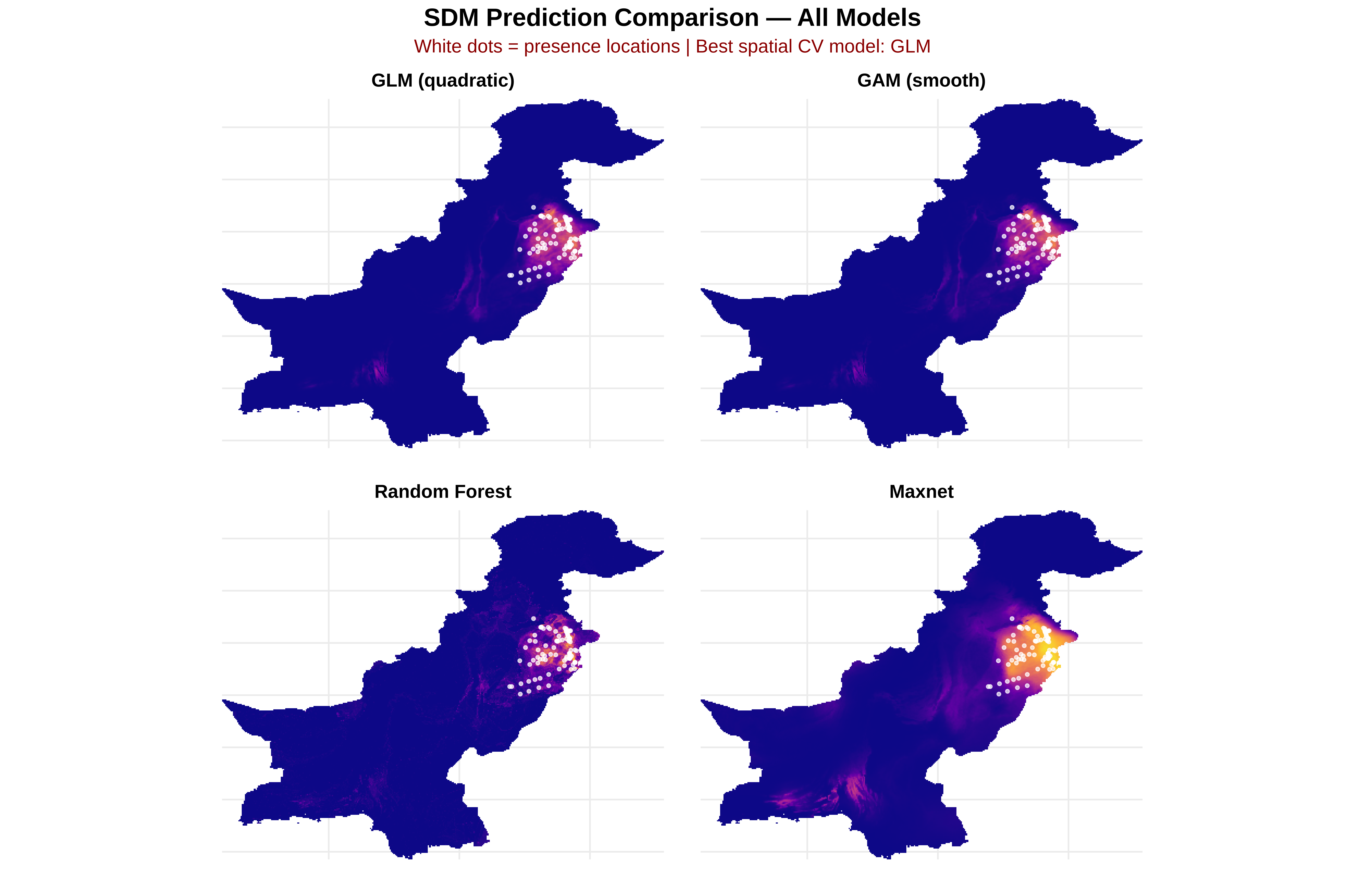
# STEP 14: RUN SPATIAL CROSS-VALIDATION ACROSS ALL MODELS
# ==============================================================================

# Helper: calculate AUC
calc_auc <- function(y, p) {
  tryCatch({
    as.numeric(pROC::auc(pROC::roc(y, p, quiet = TRUE)))
  }, error = function(e) NA_real_)
}

# Helper: fit all models and return predictions for test set
fit_and_predict <- function(train, test, pred_vars) {
  out <- list()

  # Ensure pa is factor for RF
  train$pa <- as.factor(train$pa)

  # 1. GLM (quadratic terms)
  glm_f <- as.formula(paste("pa ~",
                            paste(c(pred_vars, paste0("I(", pred_vars, "^2)")),
                                  collapse = " + ")))
  tryCatch({
    m_glm <- glm(glm_f, data = train, family = binomial)
    out$GLM <- predict(m_glm, newdata = test, type = "response")
  }, error = function(e) { out$GLM <- rep(NA, nrow(test)) })

  # 2. GAM (smooth terms)
  gam_terms <- paste0("s(", pred_vars, ", k = 4)")
  gam_f <- as.formula(paste("pa ~", paste(gam_terms, collapse = " + ")))
  tryCatch({
    m_gam <- mgcv::gam(gam_f, data = train, family = binomial, method = "REML")
    out$GAM <- predict(m_gam, newdata = test, type = "response")
  }, error = function(e) { out$GAM <- rep(NA, nrow(test)) })

  # 3. Random Forest
  tryCatch({
    m_rf <- ranger::ranger(
      as.factor(pa) ~ .,
      data = train[, c("pa", pred_vars)],
      probability = TRUE, num.trees = 400
    )
    out$RF <- predict(m_rf, data = test)$predictions[, "1"]
  }, error = function(e) { out$RF <- rep(NA, nrow(test)) })

  # 4. Maxnet
  tryCatch({
    f <- maxnet::maxnet.formula(train$pa, train[, pred_vars], classes = "lqph")
    m_mx <- maxnet::maxnet(p = train$pa, data = train[, pred_vars],
                           f = f, regmult = 1.5)
    out$Maxnet <- as.numeric(predict(m_mx, test[, pred_vars], type = "cloglog"))
  }, error = function(e) { out$Maxnet <- rep(NA, nrow(test)) })

  return(out)
}

# --- Run cross-validation ---
cat("\nRunning spatial cross-validation...\n")

cv_results <- data.frame()

for(k in sort(unique(dat$fold))) {
  cat("  Fold", k, "...")
  train <- dat %>% filter(fold != k)
  test <- dat %>% filter(fold == k)

  preds <- fit_and_predict(train, test, pred_vars)

  for(model_name in names(preds)) {
    auc_val <- calc_auc(test$pa, preds[[model_name]])
    cv_results <- rbind(cv_results, data.frame(
      fold = k, model = model_name, AUC = auc_val
    ))
    cat(paste0(" ", model_name, "=", round(auc_val, 3)))
  }
  cat("\n")
}

# --- Summarize results ---
results_summary <- cv_results %>%
  group_by(model) %>%
  summarise(
    mean_AUC = mean(AUC, na.rm = TRUE),
    sd_AUC = sd(AUC, na.rm = TRUE),
    n_folds = sum(!is.na(AUC)),
    .groups = "drop"
  ) %>%
  arrange(desc(mean_AUC))

cat("\n", paste(rep("=", 60), collapse = ""), "\n")
cat("SPATIAL CV RESULTS — MODEL COMPARISON\n")
cat(paste(rep("=", 60), collapse = ""), "\n\n")
print(as.data.frame(results_summary))

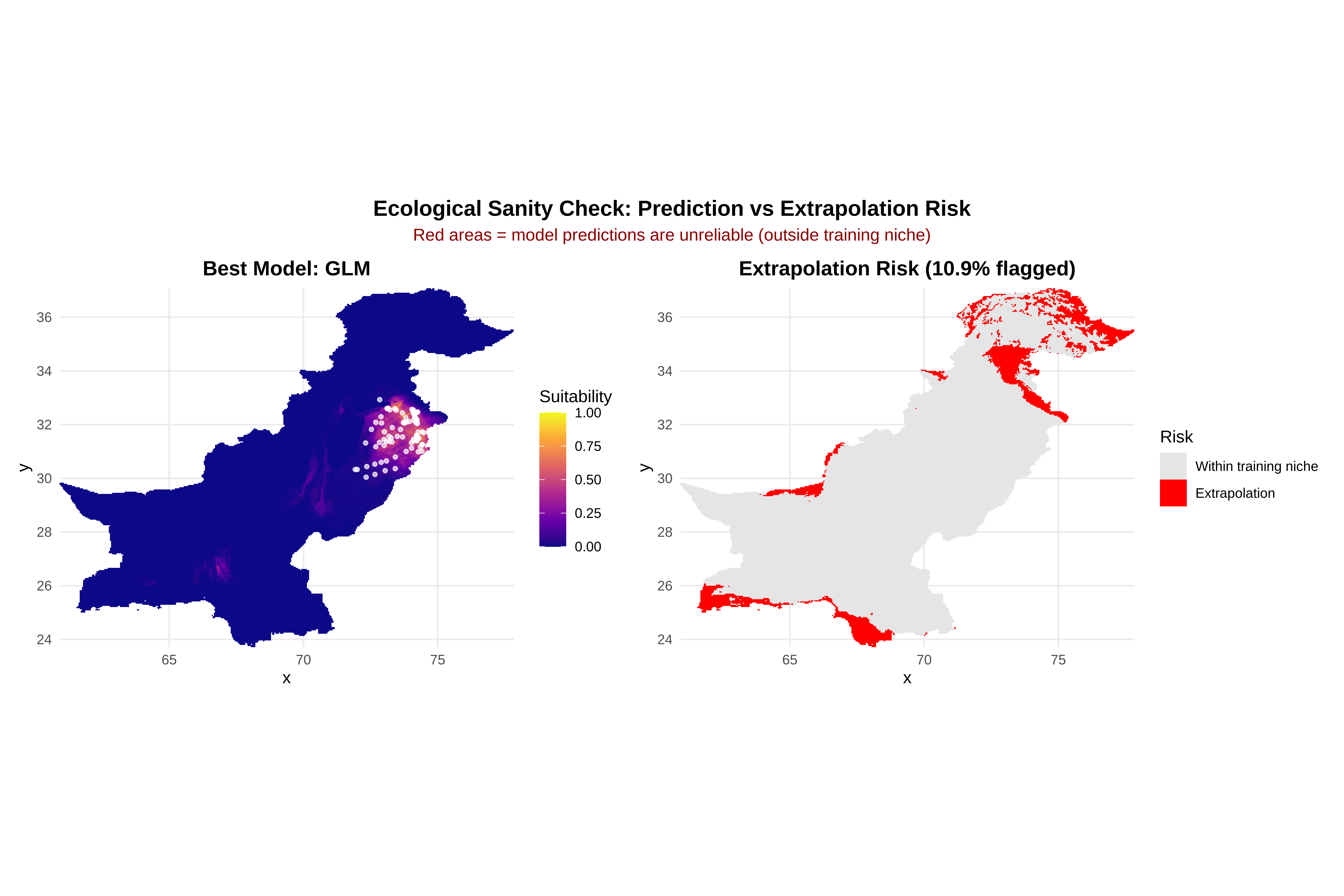
best_model_name <- results_summary$model[1]
cat("\n✓ Best model:", best_model_name,
    "(AUC =", round(results_summary$mean_AUC[1], 3),
    "±", round(results_summary$sd_AUC[1], 3), ")\n")

# ==============================================================================
# STEP 14B: FIT FINAL MODELS ON FULL DATA FOR PREDICTION
# ==============================================================================

# --- Quadratic GLM formula ---
glm_quad_formula <- as.formula(paste("pa ~",
  paste(c(pred_vars, paste0("I(", pred_vars, "^2)")), collapse = " + ")))

# --- GAM formula ---
gam_terms <- paste0("s(", pred_vars, ", k = 4)")
gam_formula <- as.formula(paste("pa ~", paste(gam_terms, collapse = " + ")))

# 1. GLM (quadratic)
glm_model <- glm(glm_quad_formula, data = dat, family = binomial)

# 2. GAM
gam_model <- mgcv::gam(gam_formula, data = dat, family = binomial, method = "REML")

# 3. Random Forest
rf_model <- ranger::ranger(
  as.factor(pa) ~ ., 
  data = dat[, c("pa", pred_vars)], 
  probability = TRUE, num.trees = 400
)

# 4. Maxnet
f <- maxnet::maxnet.formula(dat$pa, dat[, pred_vars], classes = "lqph")
maxnet_model <- maxnet::maxnet(p = dat$pa, data = dat[, pred_vars], f = f, regmult = 1.5)

cat("✓ Final models fitted on full dataset for prediction.\n")
# print(cat("✓ Final models fitted on full dataset for prediction.\n"))

Running spatial cross-validation...
  Fold 1 ... GLM=NA GAM=NA RF=NA
  Fold 2 ... GLM=NA GAM=NA RF=NA
  Fold 3 ... GLM=0.71 GAM=0.5
  Fold 4 ... GLM=NA GAM=NA RF=NA
  Fold 5 ... GLM=NA GAM=NA RF=NA

 ============================================================ 
SPATIAL CV RESULTS — MODEL COMPARISON
============================================================ 

  model  mean_AUC sd_AUC n_folds
1   GLM 0.7102072     NA       1
2   GAM 0.5000000     NA       1
3    RF       NaN     NA       0

✓ Best model: GLM (AUC = 0.71 ± NA )
✓ Final models fitted on full dataset for prediction.
Code
# ==============================================================================
# STEP 15A: VISUALISE SPATIAL CROSS-VALIDATION RESULTS
# ==============================================================================

library(ggplot2)
library(viridis)

# Boxplot + jitter for AUC values across models
p_auc <- ggplot(cv_results, aes(x = reorder(model, AUC, FUN = median),
                                y = AUC, fill = model)) +
  geom_boxplot(alpha = 0.7, width = 0.6, outlier.size = 2) +
  geom_jitter(width = 0.1, alpha = 0.4, size = 2.5) +
  stat_summary(fun = mean, geom = "point", shape = 18, size = 5, color = "black") +
  geom_hline(yintercept = 0.5, linetype = "dashed", color = "gray50") +
  annotate("text", x = 1, y = 0.52, label = "Random (AUC = 0.5)",
           hjust = 0, color = "gray50", size = 3.5) +
  scale_fill_viridis_d(option = "plasma") +
  coord_cartesian(ylim = c(0.4, 1)) +
  labs(
    title = "Spatial Cross-Validation: Model Performance",
    subtitle = paste0("Diamond = mean | ",
                      "Best: ", best_model_name, " (AUC = ",
                      round(results_summary$mean_AUC[1], 3), ")"),
    x = "", y = "AUC (Area Under ROC Curve)"
  ) +
  theme_minimal() +
  theme(
    plot.title    = element_text(hjust = 0.5, face = "bold", size = 14),
    plot.subtitle = element_text(hjust = 0.5, color = "darkred", size = 11),
    legend.position  = "none",
    panel.grid.minor = element_blank()
  )

print(p_auc)

Code
ggsave(file.path(output_path, "s5_spatial_cv_comparison.png"),
       p_auc, width = 10, height = 6, dpi = 300)
cat("✓ Step 15A complete: spatial CV plot saved.\n")


# ==============================================================================
# STEP 15B: MODEL PREDICTION AND RASTER MAPPING (Pakistan Only)
# ==============================================================================

library(terra)

# --- Map short predictor names to raster layer names ---
pred_map <- c(
  temp        = "bio1_annual_mean_temp",
  tmax        = "bio5_max_temp_warmest_month",
  temp_range  = "bio7_temp_annual_range",
  precip      = "bio12_annual_precip",
  precip_seas = "bio15_precip_seasonality"
)

# --- Subset raster stack to only predictors that exist in climate_stack ---
existing_vars <- pred_map[pred_map %in% names(climate_stack)]
missing_vars  <- setdiff(pred_map, names(climate_stack))

if (length(missing_vars) > 0) {
  warning("These predictors are missing from climate_stack and will be ignored: ",
          paste(missing_vars, collapse = ", "))
}

climate_stack_sub <- climate_stack[[existing_vars]]
names(climate_stack_sub) <- names(existing_vars)   # rename to short model variable names

# --- Prepare models ---
models      <- list(GLM = glm_model, GAM = gam_model, RF = rf_model, Maxnet = maxnet_model)
predictions <- list()

# --- Custom predict functions (terra requires signature: function(model, data, ...)) ---
pred_fun <- list(

  GLM = function(model, data, ...) {
    predict(model, as.data.frame(data), type = "response")
  },

  GAM = function(model, data, ...) {
    predict(model, as.data.frame(data), type = "response")
  },

  RF = function(model, data, ...) {
    # ranger returns a list; extract probability of class "1"
    predict(model, as.data.frame(data))$predictions[, "1"]
  },

  Maxnet = function(model, data, ...) {
    df       <- as.data.frame(data)
    out      <- rep(NA_real_, nrow(df))          # pre-fill with NAs
    complete <- complete.cases(df)               # identify non-NA rows
    if (any(complete)) {
      out[complete] <- as.numeric(
        predict(model, df[complete, , drop = FALSE], type = "cloglog")
      )
    }
    return(out)                                  # always returns nrow(df) values
  }
)

# --- Predict across Pakistan for each model ---
for (mod_name in names(models)) {
  cat("Predicting:", mod_name, "...\n")

  pred_raster <- terra::predict(
    object = climate_stack_sub,
    model  = models[[mod_name]],          # always pass model explicitly
    fun    = pred_fun[[mod_name]]         # fun must accept (model, data, ...)
  )

  # Crop & mask to Pakistan boundary
  pred_raster <- terra::crop(pred_raster, pak_boundary_vect)
  pred_raster <- terra::mask(pred_raster, pak_boundary_vect)

  # Save raster to disk
  out_file <- file.path(output_path, paste0("pred_", tolower(mod_name), "_pakistan.tif"))
  terra::writeRaster(pred_raster, out_file, overwrite = TRUE)

  # Store for plotting
  predictions[[mod_name]] <- pred_raster

  cat("  ✓ Saved:", basename(out_file), "\n")
}

cat("✓ Step 15B complete: all model predictions restricted to Pakistan and saved.\n")
✓ Step 15A complete: spatial CV plot saved.
Predicting: GLM ...
  ✓ Saved: pred_glm_pakistan.tif 
Predicting: GAM ...
  ✓ Saved: pred_gam_pakistan.tif 
Predicting: RF ...
  ✓ Saved: pred_rf_pakistan.tif 
Predicting: Maxnet ...
  ✓ Saved: pred_maxnet_pakistan.tif 
✓ Step 15B complete: all model predictions restricted to Pakistan and saved.

Interpretation Guide

AUC Range Meaning What to Expect
0.9–1.0 Excellent Rare with spatial CV; check for data leakage
0.7–0.9 Good Typical for well-performing SDMs
0.5–0.7 Poor Model barely better than random
= 0.5 Random Model has no predictive power

Key Insight: If a model scores AUC = 0.95 with random CV but only 0.70 with spatial CV, the difference is spatial autocorrelation inflation. The spatial CV result is the honest estimate of how well the model transfers to new areas.

6. Prediction Maps with Ecological Sanity Checks

Key Points:

  • Map predictions, then ask: Are hotspots plausible? Is the model extrapolating?

  • Compare multiple models visually — do they agree on core suitable areas?

  • Use extrapolation risk assessment to flag unreliable predictions

Code
# ==============================================================================
# STEP 16: GENERATE PREDICTION MAPS
# ==============================================================================
# Fit final models on ALL data, then predict across the landscape

# --- 16a: Create prediction grid ---
pred_rasters <- climate_stack[[selected_vars]]
names(pred_rasters) <- selected_short

pred_df <- as.data.frame(pred_rasters, xy = TRUE, na.rm = TRUE)

cat("Prediction grid:", nrow(pred_df), "cells\n")

# --- 16b: Fit final models on all data ---
# GLM (quadratic)
final_glm <- glm(
  as.formula(paste("pa ~",
    paste(c(pred_vars, paste0("I(", pred_vars, "^2)")), collapse = " + "))),
  data = dat, family = binomial
)

# GAM
final_gam <- gam(
  as.formula(paste("pa ~", paste(paste0("s(", pred_vars, ", k = 5)"),
                                  collapse = " + "))),
  data = dat, family = binomial, method = "REML"
)

# RF
final_rf <- ranger::ranger(
  as.factor(pa) ~ ., data = dat[, c("pa", pred_vars)],
  probability = TRUE, num.trees = 500, importance = "permutation"
)

# Maxnet
final_mx <- maxnet::maxnet(
  p = dat$pa, data = dat[, pred_vars],
  f = maxnet::maxnet.formula(dat$pa, dat[, pred_vars], classes = "lqph"),
  regmult = 1.5
)

# --- 16c: Predict ---
pred_df$GLM <- predict(final_glm, newdata = pred_df, type = "response")
pred_df$GAM <- predict(final_gam, newdata = pred_df, type = "response")
pred_df$RF <- predict(final_rf, data = pred_df)$predictions[, "1"]
pred_df$Maxnet <- as.numeric(predict(final_mx, pred_df[, pred_vars], type = "cloglog"))

cat("✓ All model predictions generated\n")

# --- 16d: Create comparison maps ---
make_map <- function(pred_df, col, title_text) {
  ggplot(pred_df, aes(x = x, y = y, fill = .data[[col]])) +
    geom_raster() +
    scale_fill_viridis_c(option = "plasma", limits = c(0, 1),
                         na.value = "transparent", name = "Suitability") +
    geom_point(data = spider_data, aes(x = X, y = Y),
               color = "white", size = 0.8, alpha = 0.7,
               inherit.aes = FALSE) +
    coord_sf(expand = FALSE) +
    labs(title = title_text, x = "", y = "") +
    theme_minimal() +
    theme(
      plot.title = element_text(hjust = 0.5, face = "bold", size = 12),
      legend.position = "none",
      axis.text = element_blank()
    )
}

p_glm_map <- make_map(pred_df, "GLM", "GLM (quadratic)")
p_gam_map <- make_map(pred_df, "GAM", "GAM (smooth)")
p_rf_map <- make_map(pred_df, "RF", "Random Forest")
p_mx_map <- make_map(pred_df, "Maxnet", "Maxnet")

p_comparison <- (p_glm_map | p_gam_map) / (p_rf_map | p_mx_map) +
  plot_annotation(
    title = "SDM Prediction Comparison — All Models",
    subtitle = paste0("White dots = presence locations | ",
                     "Best spatial CV model: ", best_model_name),
    theme = theme(
      plot.title = element_text(hjust = 0.5, face = "bold", size = 16),
      plot.subtitle = element_text(hjust = 0.5, size = 12, color = "darkred")
    )
  )

print(p_comparison)

Code
ggsave(file.path(output_path, "s5_model_comparison_maps.png"),
       p_comparison, width = 14, height = 10, dpi = 300)
Prediction grid: 48244 cells
✓ All model predictions generated
Code
# ==============================================================================
# STEP 17: EXTRAPOLATION RISK ASSESSMENT
# ==============================================================================
# Use Mahalanobis distance to identify areas outside the training niche
# This is a direct application of Session 4's climate niche space concept

# Mahalanobis distance from training data centroid
train_center <- colMeans(dat[, pred_vars])
train_cov <- cov(dat[, pred_vars])
pred_mat <- as.matrix(pred_df[, pred_vars])

maha_dist <- mahalanobis(pred_mat, train_center, train_cov)

# Chi-squared p-value: low p = outside training niche
pred_df$extrap_p <- pchisq(maha_dist, df = length(pred_vars), lower.tail = FALSE)
pred_df$extrapolation <- pred_df$extrap_p < 0.05  # Flag as risky

n_extrap <- sum(pred_df$extrapolation)
pct_extrap <- round(100 * n_extrap / nrow(pred_df), 1)

cat("\n", paste(rep("=", 60), collapse = ""), "\n")
cat("EXTRAPOLATION RISK ASSESSMENT\n")
cat(paste(rep("=", 60), collapse = ""), "\n")
cat("Cells flagged as extrapolation:", n_extrap, "/", nrow(pred_df),
    "(", pct_extrap, "%)\n")
cat("These are areas where environmental conditions fall outside\n")
cat("the multivariate training envelope (Mahalanobis p < 0.05)\n")

# Plot extrapolation map alongside best model prediction
best_col <- best_model_name

p_best_map <- ggplot(pred_df, aes(x = x, y = y, fill = .data[[best_col]])) +
  geom_raster() +
  scale_fill_viridis_c(option = "plasma", limits = c(0, 1),
                       na.value = "transparent", name = "Suitability") +
  geom_point(data = spider_data, aes(x = X, y = Y),
             color = "white", size = 1, alpha = 0.7, inherit.aes = FALSE) +
  coord_sf(expand = FALSE) +
  labs(title = paste("Best Model:", best_model_name)) +
  theme_minimal() +
  theme(plot.title = element_text(hjust = 0.5, face = "bold"))

p_extrap <- ggplot(pred_df, aes(x = x, y = y, fill = extrapolation)) +
  geom_raster() +
  scale_fill_manual(values = c("FALSE" = "gray90", "TRUE" = "red"),
                    name = "Risk",
                    labels = c("Within training niche", "Extrapolation")) +
  coord_sf(expand = FALSE) +
  labs(title = paste0("Extrapolation Risk (", pct_extrap, "% flagged)")) +
  theme_minimal() +
  theme(plot.title = element_text(hjust = 0.5, face = "bold"))

p_sanity <- p_best_map + p_extrap +
  plot_annotation(
    title = "Ecological Sanity Check: Prediction vs Extrapolation Risk",
    subtitle = "Red areas = model predictions are unreliable (outside training niche)",
    theme = theme(
      plot.title = element_text(hjust = 0.5, face = "bold", size = 14),
      plot.subtitle = element_text(hjust = 0.5, color = "darkred", size = 11)
    )
  )

print(p_sanity)

Code
ggsave(file.path(output_path, "s5_extrapolation_risk.png"),
       p_sanity, width = 12, height = 5, dpi = 300)

 ============================================================ 
EXTRAPOLATION RISK ASSESSMENT
============================================================ 
Cells flagged as extrapolation: 5269 / 48244 ( 10.9 %)
These are areas where environmental conditions fall outside
the multivariate training envelope (Mahalanobis p < 0.05)

Complete Session Summary

Code
# ==============================================================================
# STEP 18: SESSION 5 SUMMARY
# ==============================================================================

cat("\n", paste(rep("=", 70), collapse = ""), "\n")
cat("SESSION 5 SUMMARY: SPECIES DISTRIBUTION MODELING\n")
cat(paste(rep("=", 70), collapse = ""), "\n\n")

cat("1. VARIABLE SELECTION (Session 3 integration):\n")
cat("   • Started with", length(meaningful_names), "predictors\n")
cat("   • Applied VIF < 10 threshold\n")
cat("   • Final set:", paste(selected_short, collapse = ", "), "\n\n")

cat("2. MODELS FITTED:\n")
cat("   • GLM (quadratic): Parametric, interpretable\n")
cat("   • GAM (smooth):    Flexible, still interpretable\n")
cat("   • Random Forest:   Nonlinear, handles interactions\n")
cat("   • Maxnet:          MaxEnt-like, presence-background\n\n")

cat("3. SPATIAL CROSS-VALIDATION:\n")
cat("   • Method: K-means spatial blocking (", n_folds, " folds)\n")
for(i in 1:nrow(results_summary)) {
  cat(sprintf("   • %-8s: AUC = %.3f ± %.3f\n",
              results_summary$model[i],
              results_summary$mean_AUC[i],
              results_summary$sd_AUC[i]))
}
cat("   • Best model:", best_model_name, "\n\n")

cat("4. EXTRAPOLATION RISK:\n")
cat("   •", pct_extrap, "% of prediction area flagged\n")
cat("   • Predictions in flagged areas should be treated with caution\n\n")

cat("5. OUTPUT FILES:\n")
output_files <- list.files(output_path, pattern = ".png$")
for(f in output_files) cat("   ", file.path(output_path, f), "\n")

cat("\n", paste(rep("=", 70), collapse = ""), "\n")

 ====================================================================== 
SESSION 5 SUMMARY: SPECIES DISTRIBUTION MODELING
====================================================================== 

1. VARIABLE SELECTION (Session 3 integration):
   • Started with 20 predictors
   • Applied VIF < 10 threshold
   • Final set: temp, tmax, temp_range, precip, precip_seas 

2. MODELS FITTED:
   • GLM (quadratic): Parametric, interpretable
   • GAM (smooth):    Flexible, still interpretable
   • Random Forest:   Nonlinear, handles interactions
   • Maxnet:          MaxEnt-like, presence-background

3. SPATIAL CROSS-VALIDATION:
   • Method: K-means spatial blocking ( 5  folds)
   • GLM     : AUC = 0.710 ± NA
   • GAM     : AUC = 0.500 ± NA
   • RF      : AUC = NaN ± NA
   • Best model: GLM 

4. EXTRAPOLATION RISK:
   • 10.9 % of prediction area flagged
   • Predictions in flagged areas should be treated with caution

5. OUTPUT FILES:
    /run/media/tahirali/Expansion/github/spatial-ecology-workshop//output/Session_5/s5_extrapolation_risk.png 
    /run/media/tahirali/Expansion/github/spatial-ecology-workshop//output/Session_5/s5_gam_smooth_terms.png 
    /run/media/tahirali/Expansion/github/spatial-ecology-workshop//output/Session_5/s5_glm_vs_gam_response.png 
    /run/media/tahirali/Expansion/github/spatial-ecology-workshop//output/Session_5/s5_maxnet_response.png 
    /run/media/tahirali/Expansion/github/spatial-ecology-workshop//output/Session_5/s5_model_comparison_maps.png 
    /run/media/tahirali/Expansion/github/spatial-ecology-workshop//output/Session_5/s5_rf_importance.png 
    /run/media/tahirali/Expansion/github/spatial-ecology-workshop//output/Session_5/s5_spatial_cv_comparison.png 
    /run/media/tahirali/Expansion/github/spatial-ecology-workshop//output/Session_5/s5_spatial_folds.png 
    /run/media/tahirali/Expansion/github/spatial-ecology-workshop//output/Session_5/s5_vif_selection.png 
    /run/media/tahirali/Expansion/github/spatial-ecology-workshop//output/Session_5/s5_workflow.png 

 ====================================================================== 

Reasoning Prompts

Code
# ==============================================================================
# STEP 19: ECOLOGICAL REASONING PROMPTS
# ==============================================================================

cat("\n", paste(rep("=", 70), collapse = ""), "\n")
cat("REASONING PROMPTS FOR DISCUSSION\n")
cat(paste(rep("=", 70), collapse = ""), "\n\n")

cat("1. If RF beats GLM in random CV but not in spatial CV, what does that imply?\n")
cat("   → RF likely exploited spatial autocorrelation in random CV.\n")
cat("     Spatial CV removes this advantage, showing more honest performance.\n")
cat("     This is the MOST COMMON finding in SDM benchmarks.\n\n")

cat("2. If Maxnet predicts high suitability along roads, what's wrong?\n")
cat("   → Sampling bias: presences were collected near roads.\n")
cat("     Background should reflect sampling effort or accessible area.\n")
cat("     Solution: bias-corrected background or target-group background.\n\n")

cat("3. If GAM shows a unimodal temp response, does it match physiology?\n")
cat("   → Unimodal response is ecologically plausible (thermal optimum with limits).\n")
cat("     Check if the optimum matches known species biology.\n")
cat("     If the curve is monotonic, the species' range may be truncated.\n\n")

cat("4. How do you decide between VIF-selected variables vs PCA axes as predictors?\n")
cat("   → VIF selection (Session 3): Interpretable, each variable has meaning\n")
cat("   → PCA (Session 4): Uncorrelated but abstract\n")
cat("   → Compare spatial CV performance of both approaches\n")
cat("   → For publication: VIF selection is usually preferred for clarity\n\n")

cat("5. What does high extrapolation risk near mountain regions mean?\n")
cat("   → Spider sampling concentrated in lowlands (Punjab plains)\n")
cat("   → Mountain climate conditions are outside the training data\n")
cat("   → Predictions in northern Pakistan are unreliable\n")
cat("   → Need additional surveys in under-sampled environments\n")

 ====================================================================== 
REASONING PROMPTS FOR DISCUSSION
====================================================================== 

1. If RF beats GLM in random CV but not in spatial CV, what does that imply?
   → RF likely exploited spatial autocorrelation in random CV.
     Spatial CV removes this advantage, showing more honest performance.
     This is the MOST COMMON finding in SDM benchmarks.

2. If Maxnet predicts high suitability along roads, what's wrong?
   → Sampling bias: presences were collected near roads.
     Background should reflect sampling effort or accessible area.
     Solution: bias-corrected background or target-group background.

3. If GAM shows a unimodal temp response, does it match physiology?
   → Unimodal response is ecologically plausible (thermal optimum with limits).
     Check if the optimum matches known species biology.
     If the curve is monotonic, the species' range may be truncated.

4. How do you decide between VIF-selected variables vs PCA axes as predictors?
   → VIF selection (Session 3): Interpretable, each variable has meaning
   → PCA (Session 4): Uncorrelated but abstract
   → Compare spatial CV performance of both approaches
   → For publication: VIF selection is usually preferred for clarity

5. What does high extrapolation risk near mountain regions mean?
   → Spider sampling concentrated in lowlands (Punjab plains)
   → Mountain climate conditions are outside the training data
   → Predictions in northern Pakistan are unreliable
   → Need additional surveys in under-sampled environments

Session Info for Reproducibility

Code
cat("\n=== SESSION INFO ===\n")
print(sessionInfo())

=== SESSION INFO ===
R version 4.4.3 (2025-02-28)
Platform: x86_64-conda-linux-gnu
Running under: Fedora Linux 39 (Workstation Edition)

Matrix products: default
BLAS/LAPACK: /run/media/tahirali/2a4efc98-aaa3-4a01-a063-37db1463f3a8/tools/anaconda/envs/quarto-env/lib/libopenblasp-r0.3.30.so;  LAPACK version 3.12.0

locale:
 [1] LC_CTYPE=en_US.UTF-8       LC_NUMERIC=C              
 [3] LC_TIME=en_US.UTF-8        LC_COLLATE=en_US.UTF-8    
 [5] LC_MONETARY=en_US.UTF-8    LC_MESSAGES=en_US.UTF-8   
 [7] LC_PAPER=en_US.UTF-8       LC_NAME=C                 
 [9] LC_ADDRESS=C               LC_TELEPHONE=C            
[11] LC_MEASUREMENT=en_US.UTF-8 LC_IDENTIFICATION=C       

time zone: Europe/Berlin
tzcode source: system (glibc)

attached base packages:
[1] stats     graphics  grDevices utils     datasets  methods   base     

other attached packages:
 [1] MASS_7.3-65       pROC_1.19.0.1     maxnet_0.1.4      ranger_0.18.0    
 [5] mgcv_1.9-3        nlme_3.1-168      glmnet_4.1-10     Matrix_1.7-4     
 [9] car_3.1-3         carData_3.0-5     patchwork_1.3.2   viridis_0.6.5    
[13] viridisLite_0.4.2 sf_1.1-0          terra_1.8-70      tidyr_1.3.1      
[17] dplyr_1.1.4       ggplot2_4.0.0    

loaded via a namespace (and not attached):
 [1] gtable_0.3.6       shape_1.4.6.1      xfun_0.53          htmlwidgets_1.6.4 
 [5] lattice_0.22-7     vctrs_0.6.5        tools_4.4.3        generics_0.1.4    
 [9] tibble_3.3.0       proxy_0.4-27       pkgconfig_2.0.3    KernSmooth_2.23-26
[13] RColorBrewer_1.1-3 S7_0.2.0           lifecycle_1.0.4    compiler_4.4.3    
[17] farver_2.1.2       textshaping_1.0.3  codetools_0.2-20   htmltools_0.5.8.1 
[21] class_7.3-23       yaml_2.3.10        Formula_1.2-5      pillar_1.11.1     
[25] classInt_0.4-11    iterators_1.0.14   abind_1.4-8        foreach_1.5.2     
[29] tidyselect_1.2.1   digest_0.6.37      purrr_1.1.0        labeling_0.4.3    
[33] splines_4.4.3      fastmap_1.2.0      grid_4.4.3         cli_3.6.5         
[37] magrittr_2.0.4     survival_3.8-3     e1071_1.7-16       withr_3.0.2       
[41] scales_1.4.0       rmarkdown_2.30     gridExtra_2.3      ragg_1.5.0        
[45] evaluate_1.0.5     knitr_1.50         rlang_1.1.6        Rcpp_1.1.0        
[49] glue_1.8.0         DBI_1.2.3          jsonlite_2.0.0     R6_2.6.1          
[53] systemfonts_1.3.1  units_0.8-7